Session 10: Two-Tower, Multimodal Embeddings & Retrieval
“Text, ratings — and now images — all into one space. Two towers, one dot product.”
Core idea: a two-tower model learns one encoder per side that maps its input into one shared space, scored by a dot product. It’s the trick behind MF, autoencoders and Sentence-Transformers, now extended to images — and we open the vision encoder to see how a picture becomes a vector.
Source
# Setup — run this first.  (torch, sentence-transformers, scikit-image, chromadb are in the course
# .venv; the CLIP model is cached locally so this is fast and offline.)
import os, warnings; warnings.filterwarnings('ignore')
os.environ['HF_HUB_OFFLINE'] = '1'
os.environ['TRANSFORMERS_OFFLINE'] = '1'
os.environ['TRANSFORMERS_VERBOSITY'] = 'error'
os.environ['TOKENIZERS_PARALLELISM'] = 'false'
os.environ['HF_HUB_DISABLE_PROGRESS_BARS'] = '1'
import logging; logging.getLogger('sentence_transformers').setLevel(logging.ERROR)  # no encode() progress bars
from transformers.utils import logging as _hflog; _hflog.disable_progress_bar()      # no model-load progress widgets
import numpy as np
import matplotlib.pyplot as plt
from matplotlib_inline.backend_inline import set_matplotlib_formats
set_matplotlib_formats('retina')       # hi-dpi PNG: sharp like SVG, but raster — so the 14 figures don't
                                       # collide on shared SVG element IDs (glyph/clip defs) when MyST renders
                                       # them all on one page (raw inline <svg> garbles; sessions 6-9 use PNG too)
from matplotlib.patches import Rectangle, FancyBboxPatch
from PIL import Image
from skimage import data
from skimage.transform import resize
plt.rcParams.update({'figure.figsize': (12, 6), 'font.size': 13, 'axes.titlesize': 16})
BLUE, RED, GREEN, ORANGE, PURPLE, PINK = '#1976d2', '#d32f2f', '#388e3c', '#f57c00', '#7b1fa2', '#e91e63'
np.random.seed(42)

# A small, reproducible image set (scikit-image's bundled photos) — stand-ins for movie posters
# until the TMDB poster fetch is wired up. CLIP only needs PIL images.
IMG_NAMES  = ['astronaut', 'chelsea', 'coffee', 'rocket', 'hubble_deep_field', 'camera']
IMG_LABELS = ['astronaut', 'cat', 'coffee', 'rocket', 'galaxies', 'photographer']
def _as_rgb(arr):
    if arr.ndim == 2:
        arr = np.stack([arr] * 3, axis=-1)          # camera is grayscale -> 3 channels
    return Image.fromarray(arr)
IMAGES = [_as_rgb(getattr(data, n)()) for n in IMG_NAMES]

# CLIP: ONE model, encodes BOTH images and text into the SAME 512-d space (same .encode() API as S9).
from sentence_transformers import SentenceTransformer
clip = SentenceTransformer('clip-ViT-B-32')
print('CLIP ready — image & text share one 512-d space. Demo images:', ', '.join(IMG_NAMES))
CLIP ready — image & text share one 512-d space. Demo images: astronaut, chelsea, coffee, rocket, hubble_deep_field, camera
Recap: every session has been turning things into vectors
S6–7: items as content vectors (genres → cosine similarity).
S8: SVD / autoencoder learn a user & item vector from the rating matrix.
S9: neural text embeddings — any description → a vector; cold-start solved.
Today: add images, and the two-tower frame that unifies all of them.
Every method so far ends the same way: an entity becomes a point in a shared space and we compare points by dot product / cosine. Session 10 makes that frame explicit and adds a new modality — pixels — so a movie can be described by its text, its poster, and its ratings at once.
What to take home — and what to just appreciate
This is the finale: a tour of how the whole arc fits together. Read each slide at its tier.
Core — be able to explain these:
The two-tower pattern: two encoders → one shared space → a dot-product score.
A vision encoder (ViT) turns an image into a vector; CLIP puts images & text in one shared space, compared by cosine.
Evaluation: rank by embedding similarity, score it on held-out data with Recall@k / NDCG@k — and mind the popularity trap (best offline number ≠ best system).
Cold-start: content embeddings (text, and now images) can place a brand-new item; pure collaborative signal cannot.
Awareness — enjoy the idea, don’t memorize the internals: how all of these are trained (the contrastive loss & its N×N matrix, ViT objectives / MAE, SigLIP) · fusing signals into one item vector · the deeper offline-metric caveats (MNAR, online A/B).
Every slide is tagged Core or Awareness. If an Awareness slide feels dense, that’s by design — follow the picture, not every formula.
Recap (S9): how SBERT learns — contrastive training
Awareness
— the one training trick behind the whole lecture.
SBERT is trained on pairs that should mean the same: (question, its duplicate), (sentence, its paraphrase), (query, a relevant answer). Each pair is a positive.
The trick: in a batch of N pairs, each anchor’s true partner is its positive — the other N−1 partners are negatives (“in-batch negatives” — free, no extra labelling).
Score every anchor against every candidate → an N×N cosine matrix; the diagonal holds the true pairs.
Loss = softmax each row, then −log of the diagonal cell — i.e. plain cross-entropy with “the right answer is the diagonal”. It pulls the diagonal up and pushes the rest down.
Source
# Recap figure: SBERT's contrastive batch -> N x N cosine matrix; row-softmax + cross-entropy on the diagonal.
fig, ax = plt.subplots(figsize=(12.5, 6.8)); ax.axis('off')
ax.set_xlim(0, 12); ax.set_ylim(0, 8)
M = np.array([[0.90, 0.20, 0.13, 0.17],
              [0.18, 0.92, 0.16, 0.11],
              [0.15, 0.12, 0.88, 0.22],
              [0.21, 0.14, 0.19, 0.91]])
N, x0, ytop = 4, 2.3, 6.2
for r in range(N):
    for c in range(N):
        x, y = x0 + c, ytop - 1 - r
        diag = (r == c)
        fc = GREEN if diag else plt.cm.Greens(0.08 + 0.45 * M[r, c])
        ax.add_patch(Rectangle((x, y), 1, 1, facecolor=fc, edgecolor='white', lw=2))
        ax.text(x + 0.5, y + 0.5, f'{M[r, c]:.2f}', ha='center', va='center',
                fontsize=13, fontweight='bold', color='white' if diag else '#333')
for c in range(N):                                        # column = a candidate partner sentence
    ax.text(x0 + c + 0.5, ytop + 0.18, f'$B_{{{c+1}}}$', ha='center', fontsize=14, fontweight='bold', color=BLUE)
ax.text(x0 + N/2, ytop + 0.8, 'candidate partners', ha='center', fontsize=12, color=BLUE)
for r in range(N):                                        # row = an anchor sentence
    ax.text(x0 - 0.22, ytop - 1 - r + 0.5, f'$A_{{{r+1}}}$', ha='right', va='center', fontsize=14, fontweight='bold', color=GREEN)
ax.text(x0 - 0.95, ytop - N/2, 'anchor sentences', ha='center', va='center', rotation=90, fontsize=12, color=GREEN)
ax.add_patch(Rectangle((x0, ytop - 1), N, 1, fill=False, edgecolor=RED, lw=3))   # box the first row
ax.annotate('softmax this row, then take  −log(green cell)\n= cross-entropy for anchor $A_1$',
            xy=(x0 + N, ytop - 0.5), xytext=(x0 + N + 0.3, ytop - 0.5), va='center',
            fontsize=11.5, color=RED, fontweight='bold', arrowprops=dict(arrowstyle='->', color=RED, lw=1.8))
ax.text(x0 + N + 0.3, 3.5, 'diagonal = the N true pairs\n(positives — pull UP)', fontsize=11, color=GREEN, fontweight='bold', va='center')
ax.text(x0 + N + 0.3, 2.4, 'off-diagonal = in-batch\nnegatives (push DOWN)', fontsize=11, color='#777', va='center')
ax.text(6.0, 0.55, 'Exactly a classifier: for row i the "correct class" is column i.  '
        r'Cross-entropy $= -\log$ softmax of the diagonal score.',
        ha='center', fontsize=10.5, color='#333', bbox=dict(boxstyle='round', fc='#fffde7', ec='#fbc02d'))
ax.set_title('SBERT contrastive batch: N sentence pairs → an N×N cosine matrix (here N=4)', fontsize=13, fontweight='bold')
plt.tight_layout(); plt.show()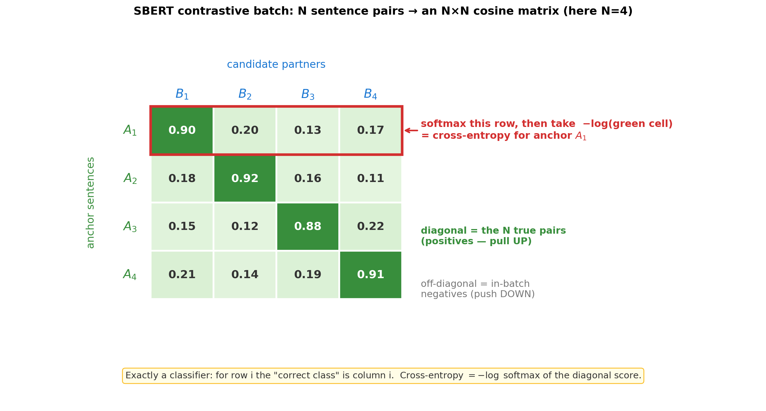
Keep this picture: two encoders → one space → pull true pairs together, push the rest apart. Today the two sides become an image and its caption (CLIP) — same matrix, same loss, just cross-modal.
The two-tower pattern
Core
— be able to explain this.
Two towers — one per side (e.g. user vs. item) — each maps its input to a vector in the same space; score = dot product of the two vectors.
Here the two towers are two different networks: an image encoder (ViT) and a text encoder (Transformer) with separate weights — the CLIP case.
Not always two networks: SBERT runs one shared encoder over both inputs; MF has no encoder at all — each tower is a plain embedding lookup.
Trained contrastively: matching pairs pulled together, mismatches pushed apart.
Source
# The two-tower pattern: two encoders -> one shared space -> dot-product score (trained contrastively).
fig, ax = plt.subplots(figsize=(12.5, 6.2)); ax.axis('off')
ax.set_xlim(0, 12); ax.set_ylim(0, 10)

def tower(x, label, inp, enc, col):
    ax.add_patch(Rectangle((x-1.3, 0.6), 2.6, 1.2, facecolor='#fff9c4', edgecolor='#f9a825', lw=2))
    ax.text(x, 1.2, inp, ha='center', va='center', fontsize=11, fontweight='bold')
    ax.add_patch(FancyBboxPatch((x-1.3, 2.6), 2.6, 1.6, boxstyle='round,pad=0.05',
                                facecolor=col, edgecolor='white', lw=2, alpha=0.92))
    ax.text(x, 3.4, enc, ha='center', va='center', fontsize=11.5, color='white', fontweight='bold')
    for j in range(4):                                   # output vector
        ax.add_patch(Rectangle((x-0.4+j*0.0, 5.1+j*0.0), 0, 0, facecolor='none'))
    for j in range(4):
        ax.add_patch(Rectangle((x-0.4, 5.0+j*0.42), 0.8, 0.42, facecolor='#e8f5e9' if col==GREEN else '#e3f2fd',
                               edgecolor=col, lw=1.4))
    ax.annotate('', xy=(x, 2.6), xytext=(x, 1.8), arrowprops=dict(arrowstyle='-|>', color='#555', lw=2))
    ax.annotate('', xy=(x, 5.0), xytext=(x, 4.2), arrowprops=dict(arrowstyle='-|>', color='#555', lw=2))
    ax.text(x, 0.2, label, ha='center', fontsize=11, fontweight='bold', color=col)

tower(2.7, 'item / image tower', 'movie poster\n(image)', 'image encoder\n(ViT)', GREEN)
tower(9.3, 'user / text tower', 'query / profile\n(text)', 'text encoder\n(Transformer)', BLUE)

# emphasise: in THIS (CLIP-style) case the two towers are genuinely different networks
ax.text(6.0, 3.4, 'two different\nnetworks\n(separate weights)', ha='center', va='center',
        fontsize=10.5, fontweight='bold', color='#333',
        bbox=dict(boxstyle='round', fc='#fffde7', ec='#fbc02d'))

# dot product node
ax.add_patch(FancyBboxPatch((5.0, 6.6), 2.0, 1.1, boxstyle='round,pad=0.06',
                            facecolor='#fffde7', edgecolor='#fbc02d', lw=2))
ax.text(6.0, 7.15, r'$\vec a \cdot \vec b$', ha='center', va='center', fontsize=16, fontweight='bold')
ax.text(6.0, 8.1, 'similarity score', ha='center', fontsize=11, color='#555')
for x0 in (2.7, 9.3):
    ax.annotate('', xy=(5.7 if x0 < 6 else 6.3, 6.9), xytext=(x0, 6.8),
                arrowprops=dict(arrowstyle='-|>', color=GREEN if x0 < 6 else BLUE, lw=2))
ax.text(6.0, 9.4, 'one shared embedding space', ha='center', fontsize=13, fontweight='bold')
ax.annotate('contrastive training: pull matching pairs together, push others apart',
            xy=(6, 5.6), ha='center', fontsize=10.5, color='#555', style='italic')
ax.set_title('Two separate encoders (image · text) → one shared space → a dot product', fontweight='bold')
plt.tight_layout(); plt.show()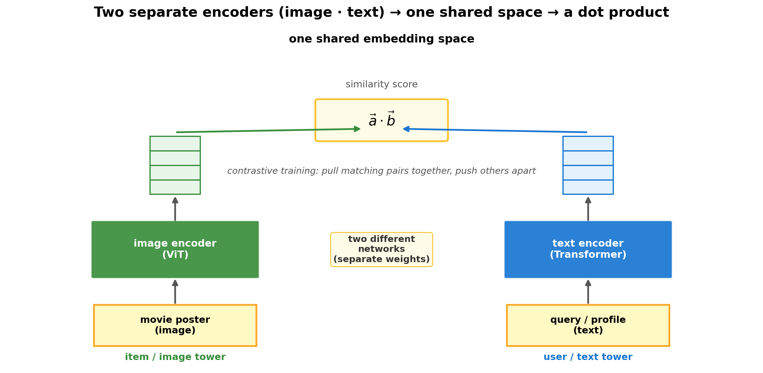
The weight-shared case counts too — SBERT is a Siamese tower (one encoder, two passes) — and even the autoencoder fits the same dot-product shape. Same shape every time.
How a vision encoder works (1): image → patches
Core
— be able to explain this.
A text encoder splits a sentence into word tokens.
A vision encoder (ViT) splits an image into a grid of patches; each patch becomes one token — the image’s version of a word token.
Each patch is flattened and linearly projected into a vector (its token / patch embedding) — just like a word vector.
Source
# Image -> a grid of patches -> a sequence of "patch tokens" (the input to a Vision Transformer).
img = resize(np.asarray(IMAGES[0]), (224, 224), anti_aliasing=True)   # the astronaut
ng = 7; P = 224 // ng                                                  # 7x7 = 49 patches of 32px
fig, (axL, axR) = plt.subplots(1, 2, figsize=(13.5, 6.0))

# left: the image with a patch grid
axL.imshow(img)
for k in range(1, ng):
    axL.axhline(k * P, color='white', lw=1.5); axL.axvline(k * P, color='white', lw=1.5)
axL.set_title(f'224×224 image, cut into {ng}×{ng} = {ng*ng} patches', fontsize=12, fontweight='bold')
axL.set_xticks([]); axL.set_yticks([])

# right: the same patches, "exploded" into a sequence with small gaps
gap = 0.28
for r in range(ng):
    for c in range(ng):
        patch = img[r*P:(r+1)*P, c*P:(c+1)*P]
        x = c * (1 + gap); y = (ng - 1 - r) * (1 + gap)
        axR.imshow(patch, extent=[x, x + 1, y, y + 1])
        axR.add_patch(Rectangle((x, y), 1, 1, fill=False, edgecolor='#90a4ae', lw=0.6))
axR.set_xlim(-0.2, ng * (1 + gap)); axR.set_ylim(-0.4, ng * (1 + gap))
axR.set_aspect('equal'); axR.axis('off')
axR.set_title(f'→ {ng*ng} patch tokens   (1 patch = 1 token)\n(flatten + linear projection → patch embeddings)',
              fontsize=12, fontweight='bold')
plt.tight_layout(); plt.show()
print('Each 32×32×3 patch is flattened to 3072 numbers, then projected to a d-dim vector — that vector is the token.')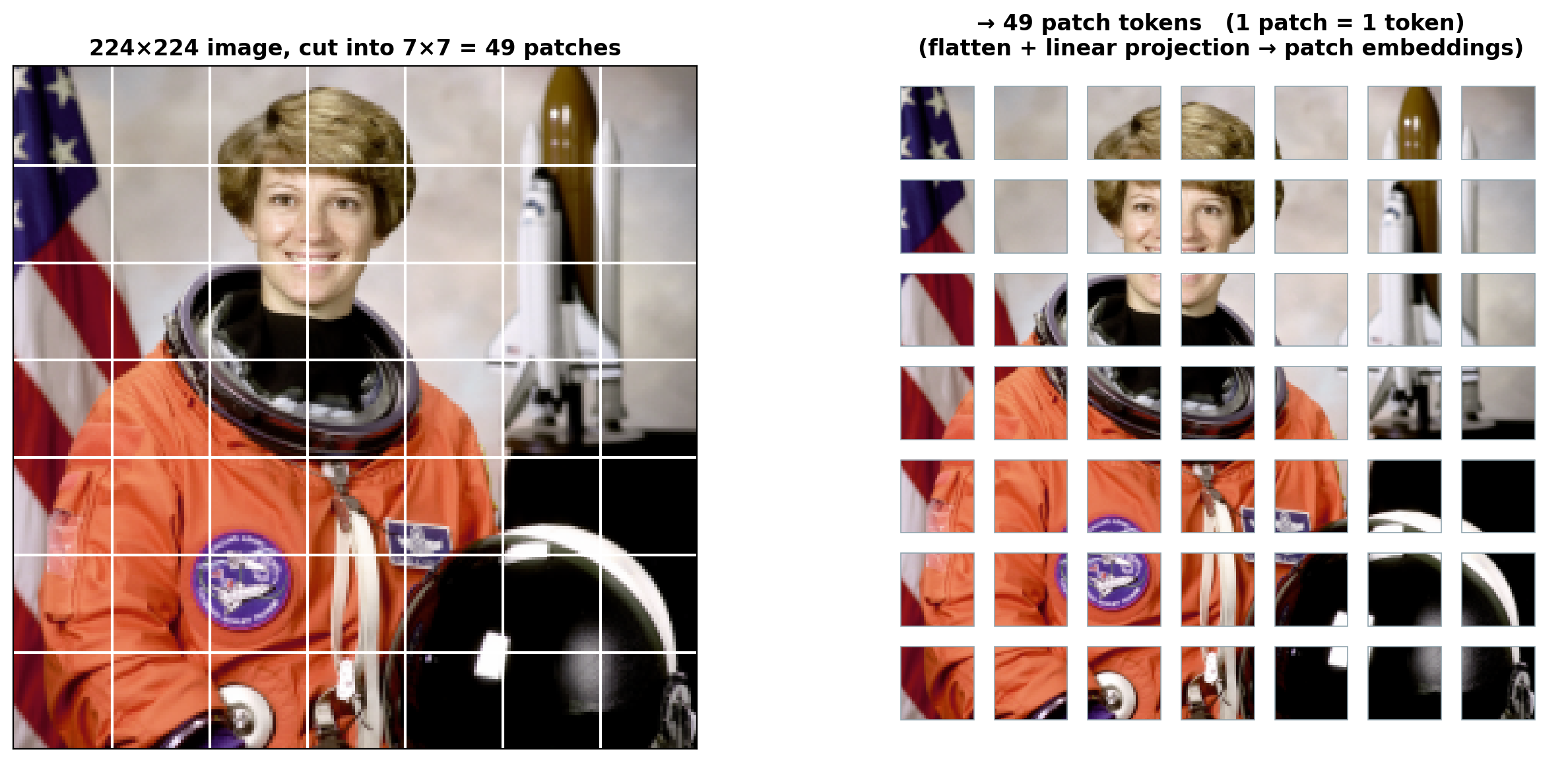
Each 32×32×3 patch is flattened to 3072 numbers, then projected to a d-dim vector — that vector is the token.
Our clip-ViT-B/32 cuts a 224×224 image into 32×32 patches → a 7×7 = 49-token sequence; each patch is flattened to 32·32·3 = 3072 numbers, then linearly projected to a d-dim vector. (Bigger ViTs, e.g. B/16, use 16×16 patches → 14×14 = 196 tokens — same idea, finer grid.) Nothing about the pixels is hand-engineered — the projection is learned, exactly like S8’s embedding matrix.
How a vision encoder works (2): patches → transformer → one vector
Core
— be able to explain this.
Add positional embeddings — self-attention treats its inputs as an unordered set, so each patch is tagged with a learned position vector (otherwise the encoder couldn’t tell top-left from bottom-right).
Run the same self-attention transformer as BERT — every patch attends to every other.
Pool the patch vectors (e.g. average them) → one image vector.
Source
# ViT pipeline drawn as a schematic, with the parallel text encoder underneath (same transformer).
# Drawn large (tall figsize + big fonts) so labels stay readable on a projector.
fig, ax = plt.subplots(figsize=(13, 6.7)); ax.axis('off')
ax.set_xlim(0, 16); ax.set_ylim(1.4, 9.2)   # crop the empty band so the pinned quote sits closer (same aspect)

def box(x, y, w, h, t, fc, ec, fs=14, fw='bold', tc='#222'):
    ax.add_patch(FancyBboxPatch((x, y), w, h, boxstyle='round,pad=0.04', facecolor=fc, edgecolor=ec, lw=2.4))
    ax.text(x + w/2, y + h/2, t, ha='center', va='center', fontsize=fs, fontweight=fw, color=tc)
def arrow(x0, x1, y):
    ax.annotate('', xy=(x1, y), xytext=(x0, y), arrowprops=dict(arrowstyle='-|>', color='#555', lw=2.6))

def token_row(x, y, n, col):
    xs = x
    for _ in range(n):
        ax.add_patch(Rectangle((xs, y), 0.5, 0.5, facecolor=col, edgecolor='white', lw=1.5))
        xs += 0.62
    return xs

# --- vision row ---
yv = 6.8
img = resize(np.asarray(IMAGES[3]), (64, 64), anti_aliasing=True)     # rocket thumbnail
ax.imshow(img, extent=[0.2, 2.0, yv - 0.35, yv + 1.5], aspect='auto', zorder=3)
ax.text(1.1, yv - 0.75, 'image', ha='center', fontsize=13, fontweight='bold', color=GREEN)
arrow(2.15, 3.0, yv + 0.6)
ax.text(2.6, yv + 1.1, 'patchify', ha='center', fontsize=12, color='#555')
xend = token_row(3.1, yv + 0.35, 6, GREEN)
ax.text((3.1 + xend)/2, yv - 0.35, 'patch tokens  + position', ha='center', fontsize=12, color='#555')
arrow(xend + 0.1, 9.3, yv + 0.6)
box(9.4, yv - 0.25, 3.0, 1.7, 'Transformer\nself-attention', PURPLE, 'white', 14, 'bold', 'white')
arrow(12.5, 13.35, yv + 0.6)
for j in range(4):
    ax.add_patch(Rectangle((13.45, yv - 0.45 + j*0.52), 0.9, 0.52, facecolor='#e8f5e9', edgecolor=GREEN, lw=1.6))
ax.text(13.9, yv + 1.95, 'image\nvector', ha='center', fontsize=12.5, fontweight='bold', color=GREEN)

# --- text row (parallel) ---
yt = 2.1
box(0.2, yt, 1.8, 1.3, '"a rocket\nlifting off"', '#e3f2fd', BLUE, 12.5, 'bold', BLUE)
arrow(2.3, 3.0, yt + 0.65)
ax.text(2.6, yt + 1.2, 'tokenize', ha='center', fontsize=12, color='#555')
xend2 = token_row(3.1, yt + 0.4, 5, BLUE)
ax.text((3.1 + xend2)/2, yt - 0.3, 'word tokens  + position', ha='center', fontsize=12, color='#555')
arrow(xend2 + 0.1, 9.3, yt + 0.65)
box(9.4, yt - 0.2, 3.0, 1.7, 'Transformer\nself-attention', PURPLE, 'white', 14, 'bold', 'white')
arrow(12.5, 13.35, yt + 0.65)
for j in range(4):
    ax.add_patch(Rectangle((13.45, yt - 0.4 + j*0.52), 0.9, 0.52, facecolor='#e3f2fd', edgecolor=BLUE, lw=1.6))
ax.text(13.9, yt + 2.0, 'text\nvector', ha='center', fontsize=12.5, fontweight='bold', color=BLUE)

ax.annotate('same encoder design, different tokenizer  →  both end as one vector in the same space',
            xy=(7.5, 5.15), ha='center', fontsize=13, color='#333', fontweight='bold',
            bbox=dict(boxstyle='round,pad=0.5', fc='#fffde7', ec='#fbc02d'))
ax.set_title('Vision Transformer = BERT for images (patches instead of words)', fontsize=15.5, fontweight='bold')
plt.tight_layout(); plt.show()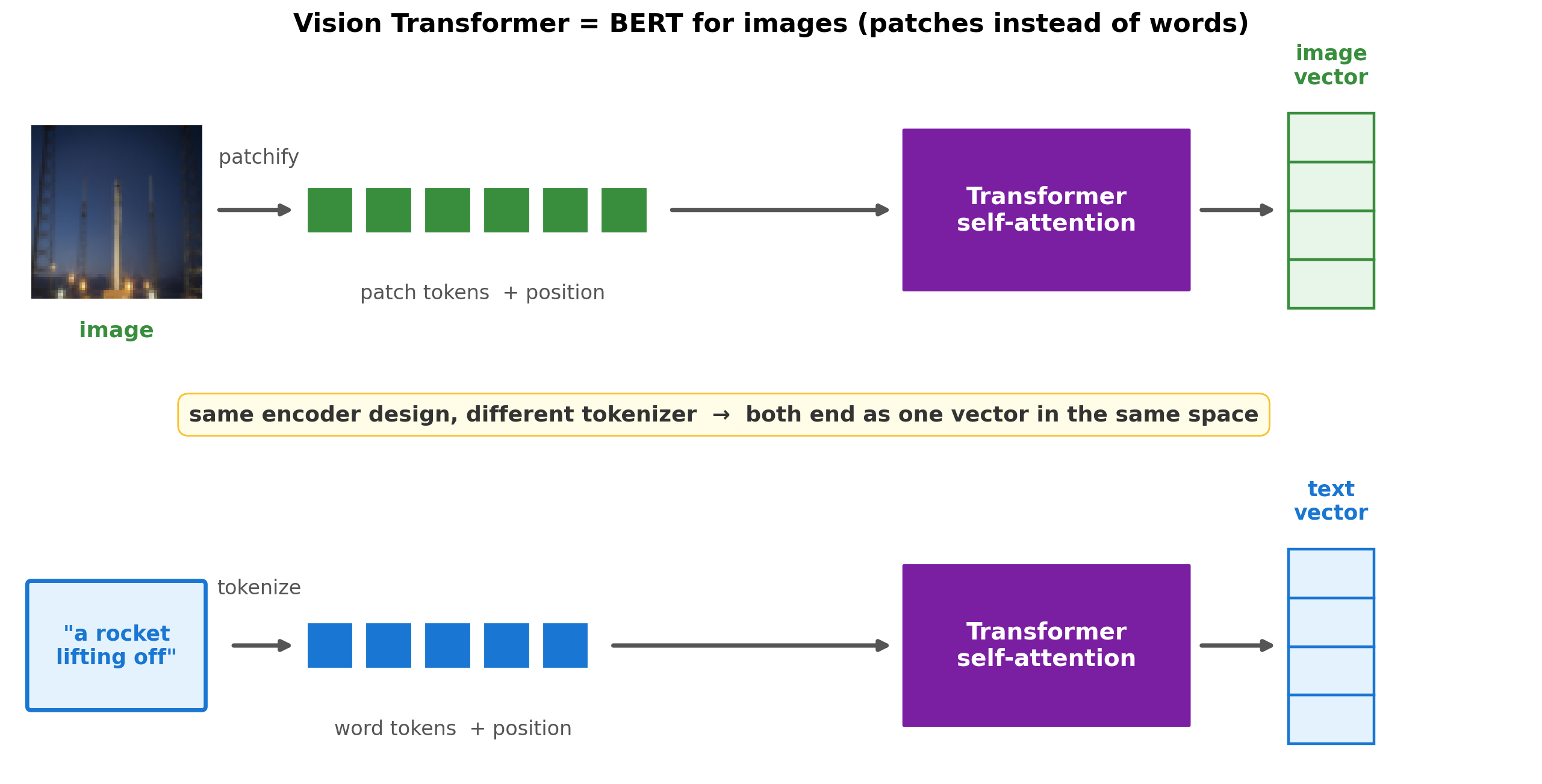
This is S9’s BERT machinery with a different tokenizer: words → patches. Because both are the same transformer, “image → vector” and “text → vector” come out as one vector of the same shape — so the two can be trained into the same space. But how do you train a ViT in the first place? (next)
How is a ViT trained? (the objective)
Awareness
— appreciate the idea, don’t memorize the internals.
BERT learns by masked tokens (fill the blank); GPT by next-token prediction. A ViT has a few options:
Supervised: add a classifier head and predict the image’s label (cat / dog / …) — the original ViT (2020).
MAE (Masked Autoencoder) — the literal “BERT for images”: hide ~70% of the patches and reconstruct them. Self-supervised, no labels — masked-token prediction, where the tokens are image patches.
Contrastive (CLIP): no labels, no reconstruction — train the image tower against captions so a picture lands next to its text. ← this is the one we use (next slide).
Source
# MAE / masked image modelling: hide most patches, reconstruct them -> the literal "BERT for images" objective.
# Single axes (deck convention) so the tight bbox stays clean.
src = resize(np.asarray(IMAGES[0]), (224, 224), anti_aliasing=True)   # astronaut
ng = 7
keep = np.random.default_rng(1).random((ng, ng)) > 0.70              # keep ~30%, hide ~70%
fig, ax = plt.subplots(figsize=(13, 5.6)); ax.axis('off')
ax.set_xlim(0, 13); ax.set_ylim(0, 7)
cell = 4.0 / ng

# left: masked input (grey over hidden patches)
ax.imshow(src, extent=[0.3, 4.3, 1.4, 5.4], aspect='auto', zorder=2)
for r in range(ng):
    for c in range(ng):
        if not keep[r, c]:
            ax.add_patch(Rectangle((0.3 + c*cell, 5.4 - (r+1)*cell), cell, cell,
                                   facecolor='#cfd8dc', edgecolor='white', lw=1, zorder=3))
ax.text(2.3, 0.85, 'input: ~70% of patches hidden', ha='center', fontsize=13, fontweight='bold')

# middle: the model + arrows (kept inside the axes)
ax.annotate('', xy=(5.4, 3.4), xytext=(4.4, 3.4), arrowprops=dict(arrowstyle='-|>', color='#555', lw=2.6))
ax.add_patch(FancyBboxPatch((5.5, 2.7), 2.0, 1.4, boxstyle='round,pad=0.05',
                            facecolor=PURPLE, edgecolor='white', lw=2))
ax.text(6.5, 3.4, 'ViT\nencoder\n+ decoder', ha='center', va='center', color='white', fontsize=12.5, fontweight='bold')
ax.annotate('', xy=(8.6, 3.4), xytext=(7.6, 3.4), arrowprops=dict(arrowstyle='-|>', color='#555', lw=2.6))
ax.text(6.5, 1.95, 'predict the\nmissing patches', ha='center', fontsize=11.5, color='#333')

# right: reconstruction target (the full image)
ax.imshow(src, extent=[8.7, 12.7, 1.4, 5.4], aspect='auto', zorder=2)
ax.text(10.7, 0.85, 'target: reconstruct the original', ha='center', fontsize=13, fontweight='bold')

ax.set_title('MAE: "masked tokens", for image patches — a ViT can learn with no labels at all',
             fontsize=14.5, fontweight='bold')
plt.tight_layout(); plt.show()
print('Other objectives: supervised (predict the label) and — what we use — contrastive against captions (CLIP, next).')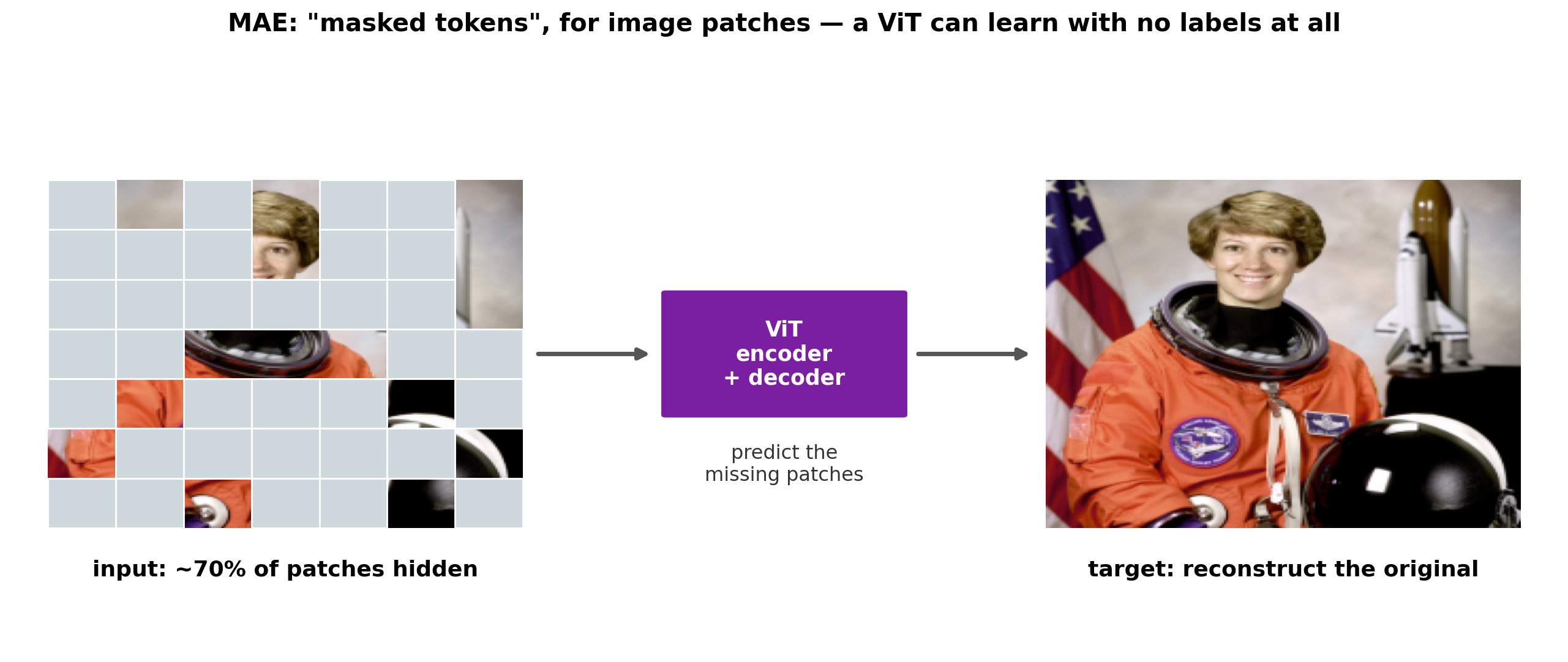
Other objectives: supervised (predict the label) and — what we use — contrastive against captions (CLIP, next).
Different objective, same backbone: however you train it, a ViT still turns an image into one vector. CLIP just trains that vector to share a space with text.
Multimodality: images and text in ONE space (CLIP)
Core
— be able to explain this.
Train an image tower (ViT) and a text tower together so a picture lands right next to its caption.
The payoff: one shared space — cosine now compares a picture and a sentence directly.
So you can write text and retrieve images (or the reverse) — meaning matches across modalities, with no shared keywords.
Source
# Concept: CLIP maps images AND text into ONE space; each photo lands next to its caption.
fig, ax = plt.subplots(figsize=(12, 6.8))
ax.set_xlim(0, 10); ax.set_ylim(0, 10)
concepts = [('astronaut', "'an astronaut'",     1.9, 7.7),
            ('cat',       "'a fluffy cat'",      7.5, 8.1),
            ('rocket',    "'a rocket launch'",   8.2, 3.1),
            ('coffee',    "'a cup of coffee'",   2.2, 2.9),
            ('galaxies',  "'distant galaxies'",  5.0, 5.4)]
for name, cap, x, y in concepts:
    ax.scatter([x], [y], marker='s', s=520, color=GREEN, edgecolor='white', linewidth=1.6, zorder=3)
    ax.scatter([x + 0.95], [y - 0.75], marker='o', s=460, color=BLUE, edgecolor='white', linewidth=1.6, zorder=3)
    ax.plot([x, x + 0.95], [y, y - 0.75], color='#bbb', lw=1.5, zorder=1)
    ax.text(x, y + 0.6, name + ' photo', ha='center', fontsize=12.5, fontweight='bold', color=GREEN)
    ax.text(x + 0.95, y - 1.4, cap, ha='center', fontsize=12.5, fontweight='bold', color=BLUE, style='italic')
ax.scatter([], [], marker='s', s=240, color=GREEN, label='image vector (ViT)')
ax.scatter([], [], marker='o', s=200, color=BLUE, label='text vector (caption)')
ax.legend(loc='upper left', frameon=False, fontsize=12.5)
ax.set_xticks([]); ax.set_yticks([])
for sp in ax.spines.values():
    sp.set_color('#ccc')
ax.text(5, 0.55, 'cosine now works ACROSS modalities: nearby = same meaning, whether image or text.',
        ha='center', fontsize=12, color='#333', bbox=dict(boxstyle='round,pad=0.5', fc='#fffde7', ec='#fbc02d'))
ax.set_title('CLIP: images and text share ONE embedding space — a photo lands next to its caption',
             fontsize=14, fontweight='bold')
plt.tight_layout(); plt.show()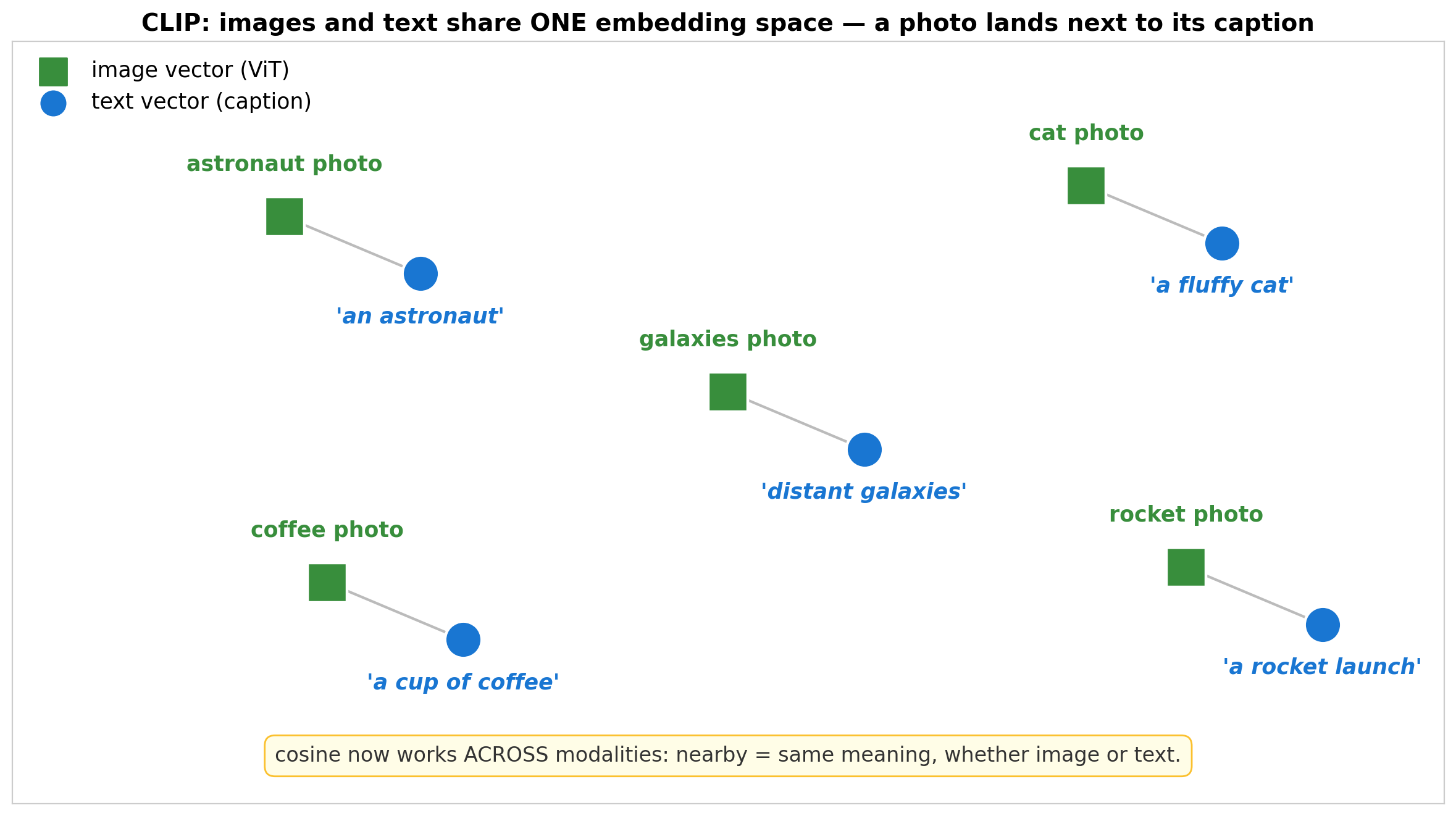
Same
SentenceTransformer.encode()as S9 — now it encodes images too, into the same 512-d space. For movies, the image tower eats posters. (CLIP, 2021; SigLIP / SigLIP-2 are the modern successors — how it’s trained is the next slide.)
How CLIP is trained: contrastive, cross-modal
Awareness
— appreciate the idea, don’t memorize the internals.
Exactly the SBERT recipe from the recap — but each positive pair is now an (image, caption).
The true pairs are the diagonal of the N×N image–text cosine matrix; push the diagonal up, the rest down.
CLIP softmaxes each row & column (InfoNCE); SigLIP instead puts an independent sigmoid on every cell (each pair judged match / no-match on its own — no batch-wide normalization, small-batch-friendly).
Source
# Teaching schematic: ONE batch -> an N x N image-text cosine matrix; training drives a bright diagonal.
fig, ax = plt.subplots(figsize=(12.5, 6.8)); ax.axis('off')
ax.set_xlim(0, 11.5); ax.set_ylim(0, 8)
M = np.array([[0.91, 0.14, 0.19, 0.08],
              [0.16, 0.88, 0.10, 0.12],
              [0.09, 0.07, 0.90, 0.21],
              [0.13, 0.18, 0.15, 0.86]])
N, x0, ytop = 4, 2.0, 6.0
for r in range(N):
    for c in range(N):
        x, y = x0 + c, ytop - 1 - r
        diag = (r == c)
        fc = GREEN if diag else plt.cm.Greens(0.08 + 0.45 * M[r, c])
        ax.add_patch(Rectangle((x, y), 1, 1, facecolor=fc, edgecolor='white', lw=2))
        ax.text(x + 0.5, y + 0.5, f'{M[r, c]:.2f}', ha='center', va='center',
                fontsize=12, fontweight='bold', color='white' if diag else '#333')
for c in range(N):                                        # column = a text/caption
    ax.text(x0 + c + 0.5, ytop + 0.18, f'$T_{{{c+1}}}$', ha='center', fontsize=13, fontweight='bold', color=BLUE)
ax.text(x0 + N/2, ytop + 0.72, 'texts / captions', ha='center', fontsize=11, color=BLUE)
for r in range(N):                                        # row = an image
    ax.text(x0 - 0.25, ytop - 1 - r + 0.5, f'$I_{{{r+1}}}$', ha='right', va='center', fontsize=13, fontweight='bold', color=GREEN)
ax.text(x0 - 0.85, ytop - N/2, 'images', ha='center', va='center', rotation=90, fontsize=11, color=GREEN)
# a row -> image-to-text loss
ax.add_patch(Rectangle((x0, ytop - 1), N, 1, fill=False, edgecolor=RED, lw=3))
ax.annotate('softmax this ROW over texts\n= L(img→txt):  image finds its caption',
            xy=(x0 + N, ytop - 0.5), xytext=(x0 + N + 0.35, ytop - 0.5), va='center',
            fontsize=10.5, color=RED, fontweight='bold', arrowprops=dict(arrowstyle='->', color=RED, lw=1.6))
# a column -> text-to-image loss
ax.add_patch(Rectangle((x0, ytop - N), 1, N, fill=False, edgecolor=BLUE, lw=3))
ax.annotate('softmax this COLUMN over images = L(txt→img):  caption finds its image',
            xy=(x0 + 0.5, ytop - N), xytext=(x0 + N/2 + 0.3, 1.4), ha='center',
            fontsize=10.5, color=BLUE, fontweight='bold', arrowprops=dict(arrowstyle='->', color=BLUE, lw=1.6))
# diagonal = positives, off-diagonal = in-batch negatives (dark-green diagonal is self-evident, no arrow)
ax.text(x0 + N + 0.35, 3.5, 'dark-green diagonal = the\nN true pairs (positives — pull UP)',
        fontsize=10, color=GREEN, fontweight='bold', va='center')
ax.text(x0 + N + 0.35, 2.4, 'off-diagonal = in-batch\nnegatives (push DOWN)', fontsize=10, color='#777', va='center')
ax.text(5.75, 0.42, 'cos(I_i, T_j) = image i vs caption j.   Train for a bright diagonal: what matters is it is the\n'
        'largest in its row & column, not its absolute value (real CLIP cosines stay modest — see next slide).',
        ha='center', fontsize=9.6, color='#333', bbox=dict(boxstyle='round', fc='#fffde7', ec='#fbc02d'))
ax.set_title('One training batch → an N×N image–text cosine matrix (here N=4)', fontweight='bold')
plt.tight_layout(); plt.show()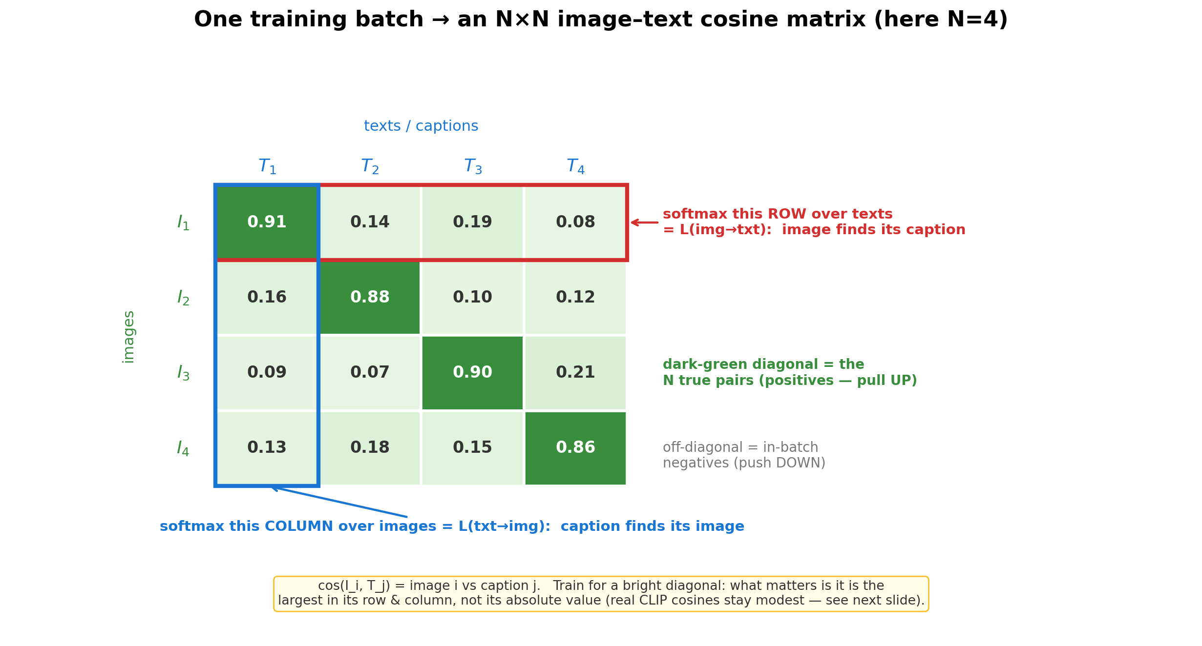
Same matrix, same loss as the S9 SBERT recap — only the two sides changed: text↔text becomes image↔text.
CLIP in action: a text query finds its image, live
Core
— be able to explain this.
The same model encodes the free-text queries and the photos; cosine ranks them.
Read each row: the query’s true image is the brightest cell (ringed) — retrieval with zero keyword overlap.
Cosines are absolute-low (~0.2–0.33) — that is by design (CLIP’s vectors all point into a narrow region of the sphere); what matters is the row-winner, not the magnitude.
# Cross-modal retrieval in a few lines: ONE model encodes BOTH images and text into one 512-d space.
from sentence_transformers import SentenceTransformer
from skimage import data
from PIL import Image

clip = SentenceTransformer('clip-ViT-B-32')            # the SAME model for images AND text

# six demo photos (skimage's bundled set) — stand-ins for movie posters
images  = [Image.fromarray(im).convert('RGB') for im in
           (data.astronaut(), data.chelsea(), data.coffee(),
            data.rocket(), data.hubble_deep_field(), data.camera())]
queries = ['an astronaut in space', 'a fluffy cat', 'a cup of coffee',
           'a rocket launch', 'a field of distant galaxies', 'a person with a camera']

iv = clip.encode(images,  normalize_embeddings=True)   # image vectors  (6 x 512)
tv = clip.encode(queries, normalize_embeddings=True)   # text  vectors  (6 x 512)
S  = tv @ iv.T                                          # cosine similarity: queries x images
Source
fig = plt.figure(figsize=(14, 6.4))
gs = fig.add_gridspec(2, len(images), height_ratios=[1, 2.4], hspace=0.35)
# top: the image thumbnails
for j, (im, lab) in enumerate(zip(images, IMG_LABELS)):
    axi = fig.add_subplot(gs[0, j]); axi.imshow(im); axi.axis('off')
    axi.set_title(lab, fontsize=10, fontweight='bold')
# bottom: the cosine heatmap, brightest cell per row ringed
axH = fig.add_subplot(gs[1, :])
axH.imshow(S, cmap='Greens', vmin=0, vmax=float(S.max()), aspect='auto')
axH.set_xticks(range(len(IMG_LABELS))); axH.set_xticklabels(IMG_LABELS, fontsize=10)
axH.set_yticks(range(len(queries))); axH.set_yticklabels(queries, fontsize=10)
for r in range(S.shape[0]):
    for c in range(S.shape[1]):
        axH.text(c, r, f'{S[r,c]:.2f}', ha='center', va='center', fontsize=9,
                 color='white' if S[r, c] > 0.55 * S.max() else '#333')
    b = int(S[r].argmax())
    axH.add_patch(Rectangle((b - 0.5, r - 0.5), 1, 1, fill=False, edgecolor=RED, lw=2.5))
axH.set_xlabel('images'); axH.set_ylabel('text queries')
axH.set_title('Text query → nearest image (red = best match). Bright diagonal = cross-modal hits.',
              fontsize=12, fontweight='bold')
plt.show()
print('One model, two modalities, one space — every query retrieves its image with no keyword overlap.')
print('Cosines look low (~0.2-0.33) by design — CLIP sharpens them with a temperature at train time; '
      'the diagonal being the row-max is the hit, not its absolute value.')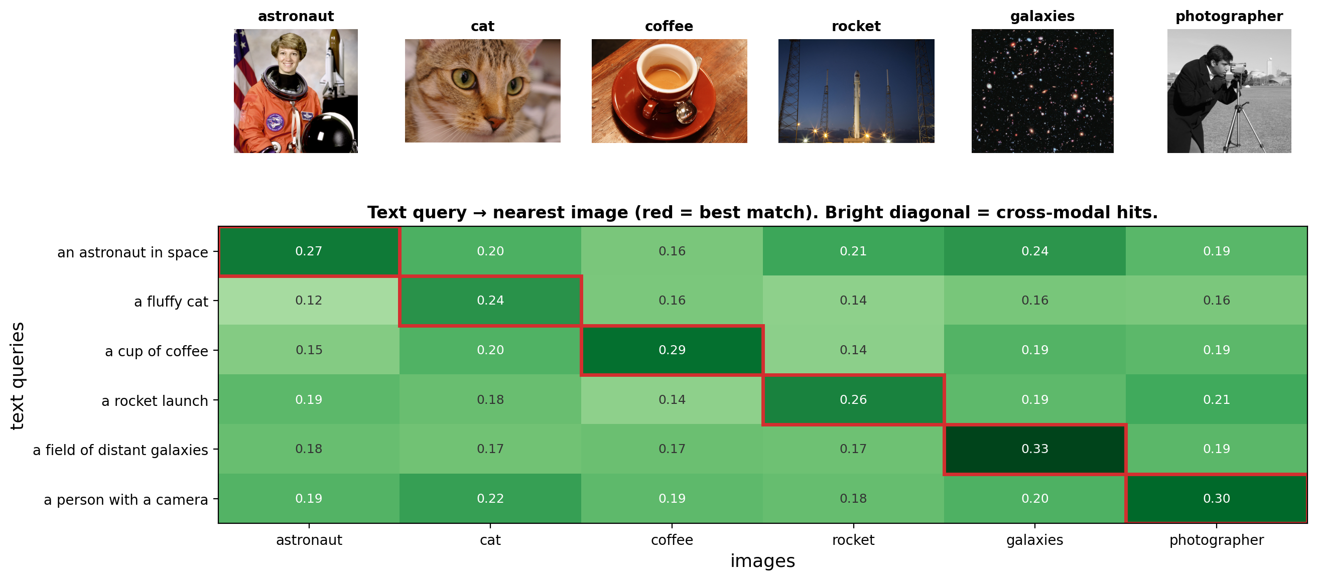
One model, two modalities, one space — every query retrieves its image with no keyword overlap.
Cosines look low (~0.2-0.33) by design — CLIP sharpens them with a temperature at train time; the diagonal being the row-max is the hit, not its absolute value.
Fusing modalities: three encoders → one item vector
Awareness
— appreciate the idea, don’t memorize the internals.
A movie has three signals — plot text, poster image, rating interactions — each with its own encoder, giving three vectors that live in different spaces and sizes.
Concatenate → a small fusion MLP → one item vector of dimension d. The fusion MLP (multi-layer perceptron — a couple of linear layers with a nonlinearity between) learns how much to trust each modality.
That item vector is scored against the user vector by the same dot product — so both towers must output the same d.
Source
# Multimodal item tower: three encoders -> concat -> fusion MLP -> ONE item vector, scored vs the user tower.
fig, ax = plt.subplots(figsize=(15, 7.8)); ax.axis('off')
ax.set_xlim(0, 16); ax.set_ylim(0, 10)

def fbox(cx, cy, w, h, t, fc, ec, fs=10, tc='#222'):
    ax.add_patch(FancyBboxPatch((cx - w/2, cy - h/2), w, h, boxstyle='round,pad=0.04',
                                facecolor=fc, edgecolor=ec, lw=2))
    if t:
        ax.text(cx, cy, t, ha='center', va='center', fontsize=fs, fontweight='bold', color=tc)

def vec(cx, cy, col, n=3, cw=0.45, ch=0.32):
    x0 = cx - (n*cw)/2
    for j in range(n):
        ax.add_patch(Rectangle((x0 + j*cw, cy - ch/2), cw, ch, facecolor=col, edgecolor='white', lw=1.2, alpha=0.92))

def arr(x0, y0, x1, y1, col='#555'):
    ax.annotate('', xy=(x1, y1), xytext=(x0, y0), arrowprops=dict(arrowstyle='-|>', color=col, lw=2))

# ---- item tower: three modality branches (left -> right), converging into the fusion block ----
rows = [('plot / overview\n(text)',      'CLIP text\nencoder',       PURPLE, 8.1, '512-d'),
        ('poster\n(image)',              'CLIP image\nencoder (ViT)', GREEN,  5.3, '512-d'),
        ('who rated it\n(interactions)', 'ID / CF\nembedding',        ORANGE, 2.5, '64-d')]
for inp, enc, col, y, dim in rows:
    fbox(1.05, y, 1.9, 1.0, inp, '#fff9c4', '#f9a825', 9.5)
    fbox(3.7, y, 2.3, 1.0, enc, col, 'white', 10, 'white')
    vec(6.0, y, col)
    ax.text(6.0, y - 0.55, dim, ha='center', fontsize=8.5, color='#555')
    arr(2.05, y, 2.55, y)
    arr(4.9, y, 5.25, y)
    arr(6.75, y, 7.05, 5.3, col)                       # converge into the fusion block

# ---- fusion block ----
fbox(8.2, 5.3, 2.2, 6.6, 'concat\n→ Fusion MLP\n(Linear→ReLU→Linear)\n→ project to d',
     '#37474f', '#263238', 10.5, 'white')
ax.text(8.2, 2.45, '512 + 512 + 64  →  d', ha='center', fontsize=8.5, color='white', style='italic')

# ---- item vector v ----
vec(10.4, 5.3, GREEN, n=4, cw=0.34, ch=0.34)
ax.text(10.4, 6.2, 'item vector  v\n(d-dim)', ha='center', fontsize=9.5, fontweight='bold', color=GREEN)
arr(9.35, 5.3, 9.68, 5.3)

# ---- dot-product node + score ----
fbox(12.2, 5.3, 1.25, 1.0, r'$\vec u \cdot \vec v$', '#fffde7', '#fbc02d', 16)
arr(11.18, 5.3, 11.55, 5.3)
arr(12.9, 5.3, 13.4, 5.3)
ax.text(14.05, 5.3, 'similarity\nscore', ha='center', va='center', fontsize=10.5, fontweight='bold', color='#333')
ax.text(12.2, 6.45, 'both towers → same dim d', ha='center', fontsize=8.8, color=RED, fontweight='bold')

# ---- user side: a faint user vector feeds the dot node from below (the full user tower is the Core slide) ----
vec(12.2, 3.7, BLUE, n=4, cw=0.5, ch=0.3)
ax.text(12.2, 2.95, 'user vector  u\n(from the user tower)', ha='center', va='center',
        fontsize=8.5, fontweight='bold', color=BLUE)
arr(12.2, 3.95, 12.2, 4.78)

# ---- CLIP shared-space callout (dashed box around the two CLIP encoders) ----
ax.add_patch(FancyBboxPatch((2.45, 4.7), 2.5, 4.0, boxstyle='round,pad=0.02',
                            fill=False, edgecolor=RED, lw=2, linestyle='--'))
ax.text(3.7, 9.0, 'CLIP already maps text + poster into ONE space',
        ha='center', fontsize=9.5, color=RED, fontweight='bold')

# ---- cold-start note ----
ax.text(3.7, 1.5, 'empty for a brand-new movie → cold start\nleans on text + poster',
        ha='center', fontsize=8.3, color='#555', style='italic')

ax.set_title('Fusing three modalities into one item vector — scored against a user vector', fontweight='bold')
plt.tight_layout(); plt.show()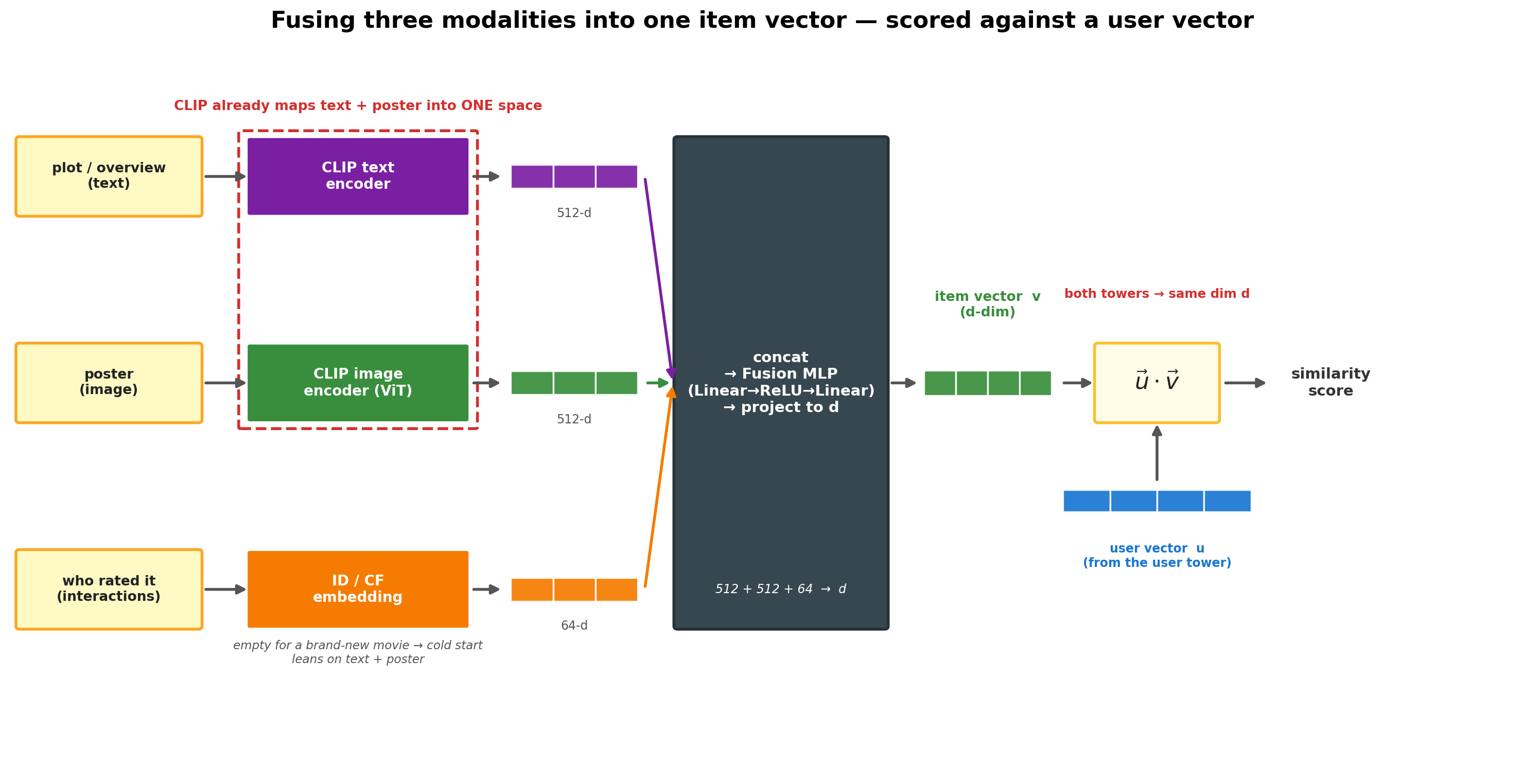
Encode text and poster with CLIP and they already share one space; the interaction branch is a separate learned table — and is empty for a brand-new movie, which is exactly why text + poster carry cold-start.
Putting it in the pipeline
Core
— the unifying idea of the whole arc.
Every tower emits a vector; the vector database (ChromaDB) doesn’t care about the modality — text, poster and ratings all become rows in the same index.
A movie can be one fused item vector (plot text + poster + interactions).
So which representation actually recommends best? Time to measure → Part 2: evaluation.
The big win of the embedding view: once everything is a vector, one retrieval engine serves content-based, collaborative and multimodal recommenders alike — and one evaluation harness scores them head-to-head.
Source
# Part 2 — evaluation harness: leave-one-out + sampled negatives, four methods. ~30s (models cached).
import pandas as pd
from sentence_transformers import SentenceTransformer
from surprise import SVD, Dataset, Reader

_rat = pd.read_csv('ml-latest-small/ratings.csv').sort_values('timestamp')
_mov = pd.read_csv('ml-latest-small/movies.csv')
EV_REL, EV_K, EV_NNEG = 4.0, 10, 100
_rng = np.random.default_rng(42)

# temporal leave-one-out: hold out each user's MOST RECENT liked (>=4) movie
_held, _prof, _seen = {}, {}, {}
for u, g in _rat.groupby('userId'):
    _seen[u] = set(g.movieId)
    pos = g[g.rating >= EV_REL]
    if len(pos) < 6:
        continue
    _held[u] = pos.movieId.iloc[-1]; _prof[u] = pos.movieId.iloc[:-1].tolist()
EV_USERS = sorted(_held)
_all = _mov.movieId.values; _mi = {m: i for i, m in enumerate(_all)}

# item features: genre one-hot (L7) + SBERT text embedding (L9)
_gs = sorted({x for gg in _mov.genres for x in gg.split('|')})
_G = np.zeros((len(_all), len(_gs)))
for _, r in _mov.iterrows():
    for x in r.genres.split('|'):
        _G[_mi[r.movieId], _gs.index(x)] = 1
_G /= (np.linalg.norm(_G, axis=1, keepdims=True) + 1e-9)
_sb = SentenceTransformer('all-MiniLM-L6-v2')
_T = _sb.encode([f"{r.title}. Genres: {r.genres.replace('|', ', ')}." for _, r in _mov.iterrows()],
                normalize_embeddings=True, show_progress_bar=False)
_pop = _rat.groupby('movieId').size().reindex(_all).fillna(0).values

# collaborative SVD (L8) trained WITHOUT the held-out positives
_ho = set((u, _held[u]) for u in EV_USERS)
_tr = _rat[~_rat[['userId', 'movieId']].apply(tuple, axis=1).isin(_ho)]
_ts = Dataset.load_from_df(_tr[['userId', 'movieId', 'rating']],
                           Reader(rating_scale=(0.5, 5))).build_full_trainset()
_svd = SVD(n_factors=50, n_epochs=20, random_state=42); _svd.fit(_ts); _mu = _ts.global_mean
def _svd_score(u, cands):
    out = np.full(len(cands), _mu)
    try:
        pu, bu = _svd.pu[_ts.to_inner_uid(u)], _svd.bu[_ts.to_inner_uid(u)]
    except Exception:
        pu, bu = None, 0.0
    for j, m in enumerate(cands):
        try:
            ii = _ts.to_inner_iid(m)
            out[j] = _mu + bu + _svd.bi[ii] + (pu @ _svd.qi[ii] if pu is not None else 0)
        except Exception:
            out[j] = -1e9                 # item with no interaction history -> CF cannot place it
    return out
def _pf(u, M):
    return M[[_mi[m] for m in _prof[u]]].mean(0)

EV_METHODS = ['Popularity', 'Content (genre)', 'Text emb (SBERT)', 'SVD (collab)']
EV_COLORS  = ['#90a4ae', GREEN, PURPLE, BLUE]
_score = {
    'Popularity':       lambda u, c: _pop[[_mi[m] for m in c]],
    'Content (genre)':  lambda u, c: _G[[_mi[m] for m in c]] @ _pf(u, _G),
    'Text emb (SBERT)': lambda u, c: _T[[_mi[m] for m in c]] @ _pf(u, _T),
    'SVD (collab)':     _svd_score,
}
def _eval(fn, only=None):
    hr = ndcg = 0.0; n = 0
    for u in EV_USERS:
        pos = _held[u]
        if only is not None and pos not in only:
            continue
        unseen = np.setdiff1d(_all, list(_seen[u]))
        negs = _rng.choice(unseen, size=min(EV_NNEG, len(unseen)), replace=False)
        cands = np.concatenate([[pos], negs]); sc = fn(u, cands)
        rank = int((sc > sc[0]).sum())              # candidates that beat the held-out positive
        if rank < EV_K:
            hr += 1; ndcg += 1 / np.log2(rank + 2)
        n += 1
    return hr / n, ndcg / n, n

_cnt = _rat.groupby('movieId').size()
EV_COLD = set(m for m in (_held[u] for u in EV_USERS) if _cnt.get(m, 0) <= 5)
ev_warm = {m: _eval(_score[m])[:2] for m in EV_METHODS}     # (Recall@k, NDCG@k)
ev_cold = {m: _eval(_score[m], only=EV_COLD)[0] for m in EV_METHODS}
EV_NCOLD = len(EV_COLD)
print('warm Recall@%d:' % EV_K, {m: round(v[0], 3) for m, v in ev_warm.items()})
print('cold Recall@%d:' % EV_K, {m: round(v, 3) for m, v in ev_cold.items()}, '| cold users:', EV_NCOLD)
warm Recall@10: {'Popularity': 0.658, 'Content (genre)': 0.262, 'Text emb (SBERT)': 0.357, 'SVD (collab)': 0.427}
cold Recall@10: {'Popularity': 0.0, 'Content (genre)': 0.237, 'Text emb (SBERT)': 0.22, 'SVD (collab)': 0.051} | cold users: 59
Part 2 — Evaluating retrieval: where’s the ground truth?
Core
— be able to explain this.
The embedding is the ranking: score every candidate by cosine similarity to the user’s profile, sort, take the top k. Content, SVD, text and multimodal all produce this same kind of ranking.
The ratings give the labels — leave-one-out: hide each user’s most-recent liked movie, then check whether the method retrieves it again (exactly how → next slide).
Two ranking metrics (here k = 10; a hit = the hidden movie reaches the top k):
Recall@k — did the hidden movie make the top k at all? With a single held-out item this is just the hit-rate: 1 if it lands in the top k, else 0.
NDCG@k — and how near the top did it land? a hit higher up is worth more, rescaled so a perfect ranking = 1 (rank 1 → 1.0, rank 3 → 0.5).
Formulas, for reference: Recall@k · NDCG@k , with and IDCG = the best-possible DCG (rescales the score into ).
Two metrics because they ask different things: Recall = did we find it, NDCG = did we rank it near the top — a method can win one and lose the other. The next slides run one identical test on every method, so the four scores are directly comparable.
How one test works — one hidden movie vs. 100 random
Core
— be able to explain this.
One trial per user: hide their most-recent liked movie (the answer), mix it into 100 random unseen movies → 101 candidates; score each against the user vector, sort, look at the top 10.
Every method is the same dot product — they differ only in how the user vector is built:
Content (L7) · Text (L9): the average of the user’s other liked-movie vectors.
SVD (L8): the learned user factor (fit from ratings, no features).
Popularity: none — it ignores the user and ranks everyone by rating count (the dumb baseline).
A hit = the hidden movie lands in the top 10; Recall@10 averages hits over users, NDCG@10 also rewards a higher rank.
Source
# How one test works: leave-one-out + sampled negatives. One user, 101 candidates -> does the hidden like reach top-10?
fig, ax = plt.subplots(figsize=(14.5, 7.4)); ax.axis('off')
ax.set_xlim(0, 16); ax.set_ylim(0, 10)
GOLD = '#f9a825'

def fbox(cx, cy, w, h, t, fc, ec, fs=10, tc='#222', lw=2.0):
    ax.add_patch(FancyBboxPatch((cx - w/2, cy - h/2), w, h, boxstyle='round,pad=0.04',
                                facecolor=fc, edgecolor=ec, lw=lw))
    if t:
        ax.text(cx, cy, t, ha='center', va='center', fontsize=fs, fontweight='bold', color=tc)

def arr(x0, y0, x1, y1, col='#555', lw=2.0):
    ax.annotate('', xy=(x1, y1), xytext=(x0, y0), arrowprops=dict(arrowstyle='-|>', color=col, lw=lw))

# ---- candidate pool (top centre): 1 hidden + 100 random ----
ax.text(8.0, 9.5, '101 candidates  =  1 hidden liked movie  +  100 random unseen', ha='center',
        fontsize=12, fontweight='bold', color='#333')
fbox(5.9, 8.5, 2.5, 0.6, 'hidden liked movie', GOLD, 'white', 9.5, 'white')
ax.text(5.9, 7.95, 'the one we removed = the answer', ha='center', fontsize=8.3, color='#a06800')
for r in range(3):
    for c in range(10):
        ax.add_patch(Rectangle((7.6 + c*0.3, 8.0 + r*0.3), 0.24, 0.24,
                               facecolor='#cfd8dc', edgecolor='white', lw=0.7))
ax.text(9.1, 7.7, '100 random unseen (negatives)', ha='center', fontsize=8.3, color='#777')
arr(7.9, 7.45, 7.9, 6.1)

# ---- user vector (left) ----
fbox(2.35, 8.3, 0.7, 0.55, '', '#cfd8dc', '#90a4ae', lw=1.4)
fbox(3.05, 8.3, 0.7, 0.55, '', '#cfd8dc', '#90a4ae', lw=1.4)
fbox(2.70, 7.65, 0.7, 0.55, '', '#cfd8dc', '#90a4ae', lw=1.4)
ax.text(2.7, 6.85, "user's other\nliked movies", ha='center', fontsize=8.6, color='#555')
arr(2.7, 6.45, 2.7, 5.85, BLUE)
fbox(2.7, 5.35, 2.3, 0.9, 'user vector  u', BLUE, 'white', 12, 'white')
arr(3.9, 5.35, 6.4, 5.35, BLUE)

# ---- scoring engine (centre): both inputs meet here ----
fbox(8.0, 5.35, 3.0, 1.5, 'score every candidate\nagainst  u  (dot product)\n-> sort', '#37474f', '#263238', 11, 'white')
arr(9.55, 5.35, 11.05, 5.35, GREEN)

# ---- sorted top-10 window (right) ----
wcx = 13.45
fbox(wcx, 4.6, 3.0, 6.5, '', '#ffffff', GREEN, lw=2.2)
ax.text(wcx, 7.95, 'sorted  -  TOP 10', ha='center', fontsize=9.5, fontweight='bold', color=GREEN)
for i in range(10):
    y = 7.4 - i*0.55
    hit = (i == 2)
    fbox(wcx + 0.15, y, 2.35, 0.45, '', GOLD if hit else '#eceff1', '#f9a825' if hit else '#cfd8dc', lw=1.1)
    ax.text(wcx - 1.2, y, str(i + 1), ha='center', va='center', fontsize=8, color='#888')
    if hit:
        ax.text(wcx + 0.15, y, 'hidden movie', ha='center', va='center', fontsize=8.5, fontweight='bold', color='white')
ax.text(wcx, 1.5, 'ranks 11 ... 101  (the rest)', ha='center', fontsize=8.3, color='#aaa')
hy = 7.4 - 2*0.55
ax.text(wcx + 2.05, hy, 'in top 10\n-> HIT', ha='center', va='center', fontsize=9.5, fontweight='bold', color=GREEN)

# ---- where u comes from (bottom-left note) ----
fbox(4.3, 2.55, 7.4, 2.1, '', '#f5f5f5', '#bdbdbd', lw=1.4)
note = ("where  u  comes from  -  the ONLY thing that differs between methods:\n"
        "    Content (L7) / Text (L9):   average of the user's liked-movie vectors\n"
        "    SVD (L8):   learned user factor  p_u   (fit from ratings, no features)\n"
        "    Popularity:   none  -  ranks everyone by rating count (the dumb baseline)")
ax.text(0.75, 3.35, note, ha='left', va='top', fontsize=9.3, color='#333')

# ---- bottom caption ----
ax.text(8.0, 0.55,
        'Recall@10 = fraction of users whose hidden movie reaches the top 10  (one trial per user, averaged).   '
        'NDCG@10 also rewards a higher rank.', ha='center', fontsize=9.8, color='#333')
plt.tight_layout(); plt.show()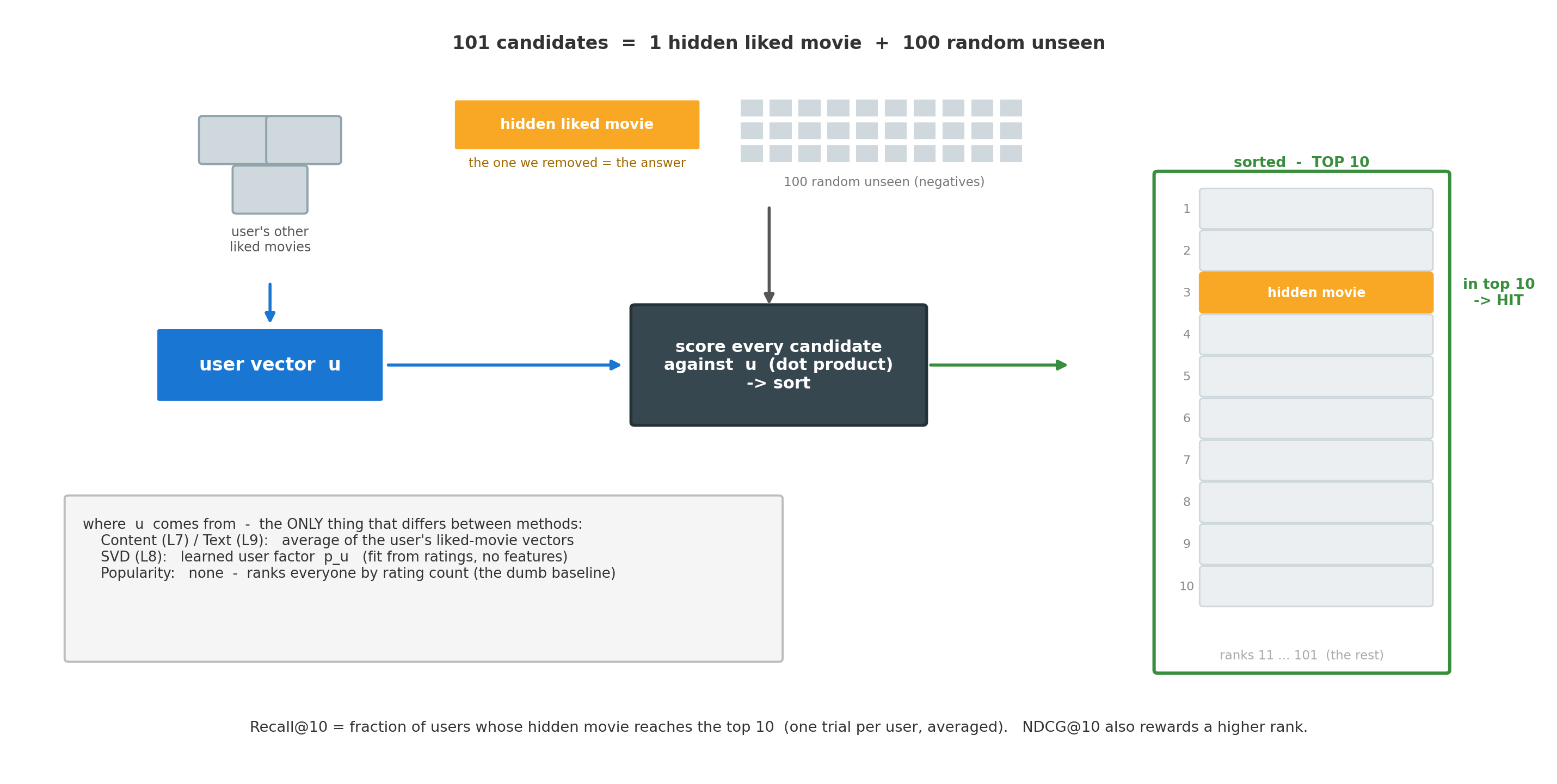
One yardstick for all four. Two more methods (autoencoder, fusion MLP) need a trained network — next slide — then the leaderboard, where the dumbest method wins anyway.
Two methods we left out — where their user vector comes from
Awareness
— appreciate the idea, don’t memorize the internals.
The four methods on the leaderboard build the user vector cheaply, with no training — an average of liked-movie vectors (content, text), a learned factor read straight from the rating matrix (SVD), or nothing at all (popularity).
Two more methods fit the exact same dot product, but their user vector is the output of a trained neural network — so we’d need fitted weights to score them:
Autoencoder (S8 / S9): the user vector is the learned decoder row (the movie side is the computed bottleneck ); the score is .
Fusion MLP / two-tower (today): the user vector is the output of a separate, learned user tower (the item side is the fused multimodal vector).
We have no trained weights for these on MovieLens, so they sit out of our leaderboard — but they’d plug into the exact same hidden-movie test.
Source
# Two more methods fit the SAME dot product, but their user vector is the output of a TRAINED network --
# we have no such weights fitted on MovieLens, so they sit out of the leaderboard.
fig, ax = plt.subplots(figsize=(14.5, 6.6)); ax.axis('off')
ax.set_xlim(0, 15); ax.set_ylim(0, 9)
RED2 = '#d32f2f'

def box(cx, cy, w, h, t, fc, ec, fs=10, tc='#222', lw=1.8):
    ax.add_patch(FancyBboxPatch((cx - w/2, cy - h/2), w, h, boxstyle='round,pad=0.04',
                                facecolor=fc, edgecolor=ec, lw=lw))
    if t:
        ax.text(cx, cy, t, ha='center', va='center', fontsize=fs, fontweight='bold', color=tc)

def arr(x0, y0, x1, y1, col='#666', lw=1.8):
    ax.annotate('', xy=(x1, y1), xytext=(x0, y0), arrowprops=dict(arrowstyle='-|>', color=col, lw=lw))

# ---- two dashed (= excluded) panels ----
ax.add_patch(FancyBboxPatch((0.3, 1.5), 7.0, 6.0, boxstyle='round,pad=0.02',
                            fill=False, edgecolor='#9e9e9e', lw=2, linestyle='--'))
ax.add_patch(FancyBboxPatch((7.7, 1.5), 7.0, 6.0, boxstyle='round,pad=0.02',
                            fill=False, edgecolor='#9e9e9e', lw=2, linestyle='--'))
ax.text(3.8, 8.5, 'Autoencoder  (S8 / S9)', ha='center', fontsize=12.5, fontweight='bold', color='#333')
ax.text(11.2, 8.5, 'Fusion MLP / two-tower  (today)', ha='center', fontsize=12.5, fontweight='bold', color='#333')
for cx in (3.8, 11.2):
    ax.text(cx, 7.85, 'trained model -- no weights on our data -> left out of the leaderboard',
            ha='center', fontsize=8.6, color=RED2, fontweight='bold')

# ===== LEFT: Autoencoder -- user vector = learned decoder row V_u =====
hx, hy = 1.1, 6.3
for j in range(4):
    ax.add_patch(Rectangle((hx, hy - j*0.5), 0.5, 0.5, facecolor='#ffebee', edgecolor=RED2, lw=1.6))
ax.text(hx + 0.25, hy + 0.45, r'$h_i$', ha='center', color=RED2, fontsize=13, fontweight='bold')
ax.text(hx + 0.25, hy - 4*0.5 - 0.3, 'movie\n(computed)', ha='center', color=RED2, fontsize=8.5)
vx, vy, rows, cols, uhi = 3.0, 6.55, 5, 4, 2
for r in range(rows):
    for c in range(cols):
        fc = '#e8f5e9' if r == uhi else '#f4f4f4'
        ax.add_patch(Rectangle((vx + c*0.5, vy - (r+1)*0.5), 0.5, 0.5, facecolor=fc, edgecolor='#bbb', lw=0.8))
ax.add_patch(Rectangle((vx, vy - (uhi+1)*0.5), cols*0.5, 0.5, fill=False, ec=GREEN, lw=2.4))
ax.text(vx + cols*0.5/2, vy + 0.3, r'decoder $V$', ha='center', fontsize=9.5, fontweight='bold')
ax.text(vx + cols*0.5 + 0.2, vy - (uhi+0.5)*0.5, r'row $u = V_u$', ha='left', color=GREEN, fontsize=10, fontweight='bold')
box(3.8, 2.7, 6.0, 1.0, '', '#e8f5e9', GREEN, lw=1.8)
ax.text(3.8, 2.95, 'user vector  =  learned decoder row  $V_u$', ha='center', fontsize=10.5, fontweight='bold', color=GREEN)
ax.text(3.8, 2.45, r'score  $\hat r_{ui} = h_i \cdot V_u$  (same dot product)', ha='center', fontsize=9.5, color='#444')

# ===== RIGHT: Fusion MLP -- user vector = output of a learned user tower =====
mods = [('text', PURPLE, 6.8), ('poster', GREEN, 6.0), ('interactions', ORANGE, 5.2)]
for t, col, y in mods:
    box(8.6, y, 1.35, 0.6, t, col, 'white', 8.5, 'white')
    arr(9.3, y, 9.9, 6.0, col)
box(10.7, 6.0, 1.45, 1.8, 'fusion\nMLP', '#37474f', '#263238', 9.5, 'white')
arr(11.45, 6.0, 12.0, 6.0, '#555')
for j in range(4):
    ax.add_patch(Rectangle((12.1 + j*0.3, 5.85), 0.26, 0.3, facecolor=GREEN, edgecolor='white', lw=1))
ax.text(12.7, 6.45, 'item vector  v', ha='center', fontsize=8.8, fontweight='bold', color=GREEN)
box(10.7, 3.7, 2.1, 0.85, 'user tower\n(learned net)', BLUE, 'white', 9, 'white')
arr(11.75, 3.7, 12.05, 3.7, BLUE)
for j in range(4):
    ax.add_patch(Rectangle((12.1 + j*0.3, 3.55), 0.26, 0.3, facecolor=BLUE, edgecolor='white', lw=1))
ax.text(12.7, 4.15, 'user vector  u', ha='center', fontsize=8.8, fontweight='bold', color=BLUE)
box(11.2, 2.4, 6.2, 0.8, 'user vector  u  =  output of a learned user tower', '#e3f2fd', BLUE, 9.4, BLUE, lw=1.8)

# ---- bottom caption ----
ax.text(7.5, 0.75,
        'Both fit the very same dot product and plug into the exact same hidden-movie test -- we just have no '
        'trained weights for them on MovieLens, so they are out of THIS leaderboard.',
        ha='center', fontsize=9.5, color='#333')
plt.tight_layout(); plt.show()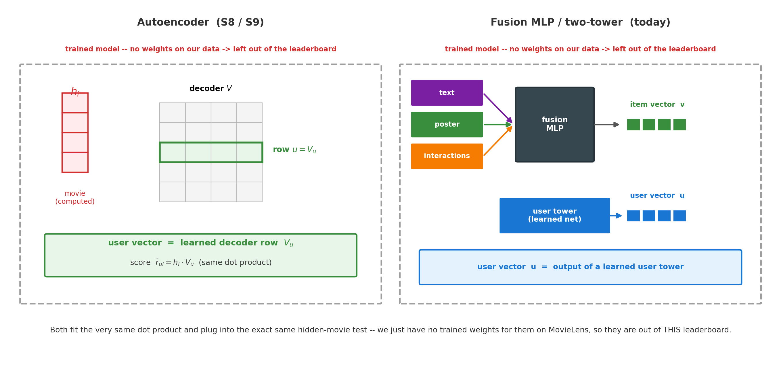
Same dot product every time — only the source of the two vectors changes. Now the four methods we can score go head-to-head on the leaderboard.
The leaderboard — and a trap
Core
— be able to explain this.
Same task as the last slide, four rankers. Each method sorts the 101 candidates (the 1 hidden liked movie + 100 random ones); we check whether the hidden movie reaches the top 10.
The four methods:
Popularity — rank by a movie’s total number of ratings (most-rated first). The same list for everyone — no personalization (our dumb baseline).
Content (L7) · Text (L9) · SVD (L8) — the personalized methods from earlier sessions.
The trap: the dumbest method — popularity — wins the raw Recall@10 (chart).
Source
# Warm-start leaderboard: 4 methods on the x-axis, 2 bars each coloured BY METRIC (so the legend matches).
fig, ax = plt.subplots(figsize=(12.5, 5.6))
x = np.arange(len(EV_METHODS)); w = 0.38
rec = [ev_warm[m][0] for m in EV_METHODS]; ndg = [ev_warm[m][1] for m in EV_METHODS]
b1 = ax.bar(x - w/2, rec, w, label=f'Recall@{EV_K}  (= hit-rate)', color=BLUE, edgecolor='white')
b2 = ax.bar(x + w/2, ndg, w, label=f'NDCG@{EV_K}', color=ORANGE, edgecolor='white')
for b in list(b1) + list(b2):
    ax.text(b.get_x() + b.get_width()/2, b.get_height() + 0.012, f'{b.get_height():.2f}',
            ha='center', fontsize=9)
ax.set_xticks(x); ax.set_xticklabels(EV_METHODS); ax.set_ylim(0, max(rec) * 1.28)
ax.set_ylabel('score'); ax.legend(loc='upper right', frameon=False, title='metric')
ax.spines[['top', 'right']].set_visible(False)
ax.set_title(f'Warm-start: rank 1 hidden liked movie among {EV_NNEG} random others (all users)', fontweight='bold')
ax.annotate('popularity wins?!', xy=(0, rec[0]), xytext=(0.7, rec[0] + 0.11),
            fontsize=11, color=RED, fontweight='bold', ha='center',
            arrowprops=dict(arrowstyle='->', color=RED, lw=1.8))
plt.tight_layout(); plt.show()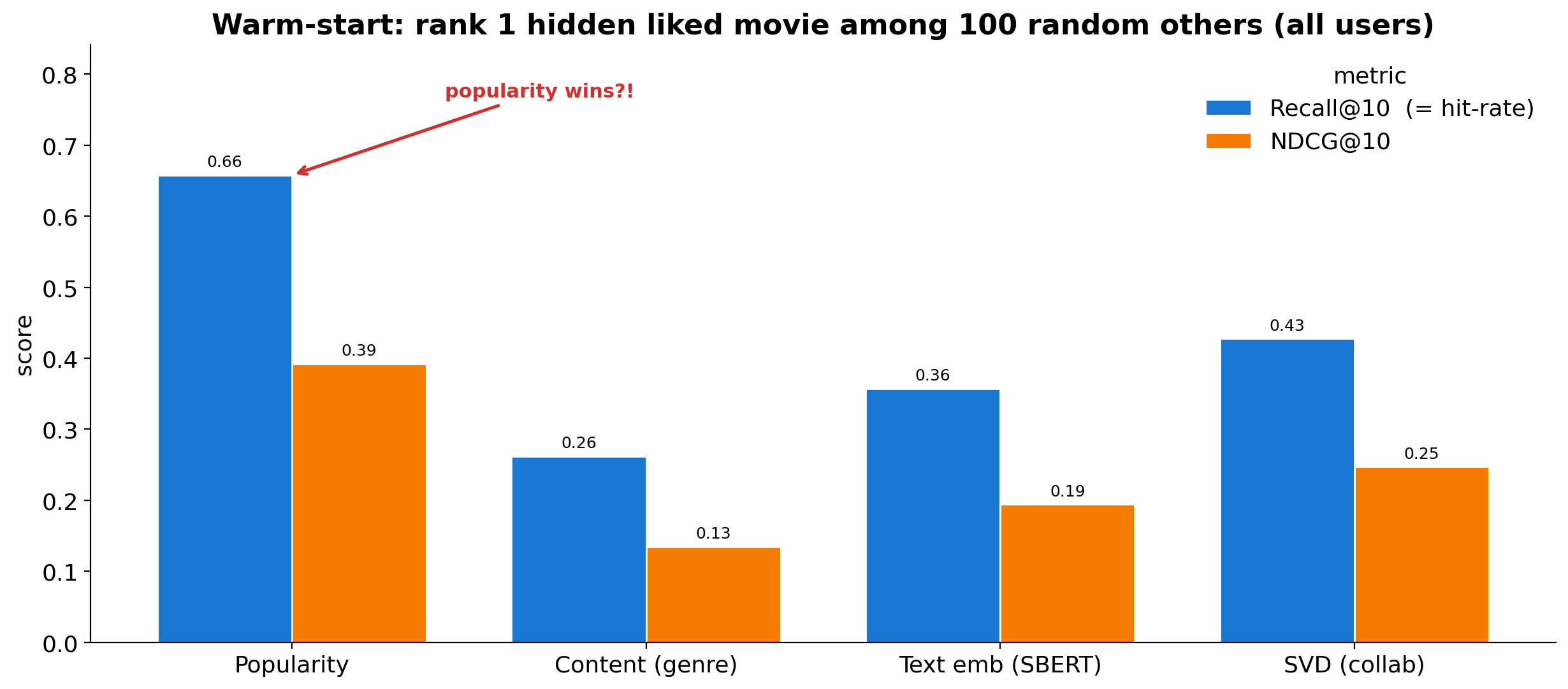
A held-out liked movie is usually itself popular, so against random negatives the popularity baseline ranks it high — so sampled-negative metrics flatter popularity, and sampled scores can even reorder which method “wins” versus a full-catalogue ranking. Best offline number ≠ best system. Personalization earns its keep on diversity, the long tail, and — next slide — cold-start.
Refs — Cremonesi, Koren & Turrin, Performance of Recommender Algorithms on Top-N Recommendation Tasks , RecSys 2010 ( Cremonesi et al. (2010) ) · Krichene & Rendle, On Sampled Metrics for Item Recommendation , KDD 2020 ( research.google ).
Cold-start: the real test
Core
— be able to explain this.
Re-run the exact same test, but only on the sparse items (≤5 ratings) — the new-release case.
Popularity and collaborative SVD collapse (no ratings to lean on); content & text embeddings hold up (they place the item from its features, not its history). Same four methods, warm vs cold.
Source
# The real test: warm vs COLD-start Recall@10. Collaborative methods collapse; content/text survive.
fig, ax = plt.subplots(figsize=(12.5, 5.8))
x = np.arange(len(EV_METHODS)); w = 0.38
warm = [ev_warm[m][0] for m in EV_METHODS]; cold = [ev_cold[m] for m in EV_METHODS]
ax.bar(x - w/2, warm, w, label='warm  (popular hidden movie)', color='#b0bec5', edgecolor='white')
ax.bar(x + w/2, cold, w, label=f'cold  (≤5-rating movie, n={EV_NCOLD})', color=BLUE, edgecolor='white')
for i, (wv, cv) in enumerate(zip(warm, cold)):
    ax.text(i - w/2, wv + 0.012, f'{wv:.2f}', ha='center', fontsize=9)
    ax.text(i + w/2, cv + 0.012, f'{cv:.2f}', ha='center', fontsize=9)
ax.set_xticks(x); ax.set_xticklabels(EV_METHODS); ax.set_ylabel(f'Recall@{EV_K}')
ax.set_ylim(0, max(warm) * 1.28); ax.legend(loc='upper right', frameon=False)
ax.spines[['top', 'right']].set_visible(False)
ax.set_title('Cold-start is the real test: collaborative signal vanishes, content/text survive',
             fontweight='bold')
ax.annotate('collapse', xy=(0 + w/2, cold[0]), xytext=(0.05, 0.22), ha='center', color=RED,
            fontsize=10.5, fontweight='bold', arrowprops=dict(arrowstyle='->', color=RED, lw=1.8))
ax.annotate('survive', xy=(1 + w/2, cold[1]), xytext=(1 + w/2, cold[1] + 0.13), ha='center',
            color=GREEN, fontsize=10.5, fontweight='bold',
            arrowprops=dict(arrowstyle='->', color=GREEN, lw=1.8))
plt.tight_layout(); plt.show()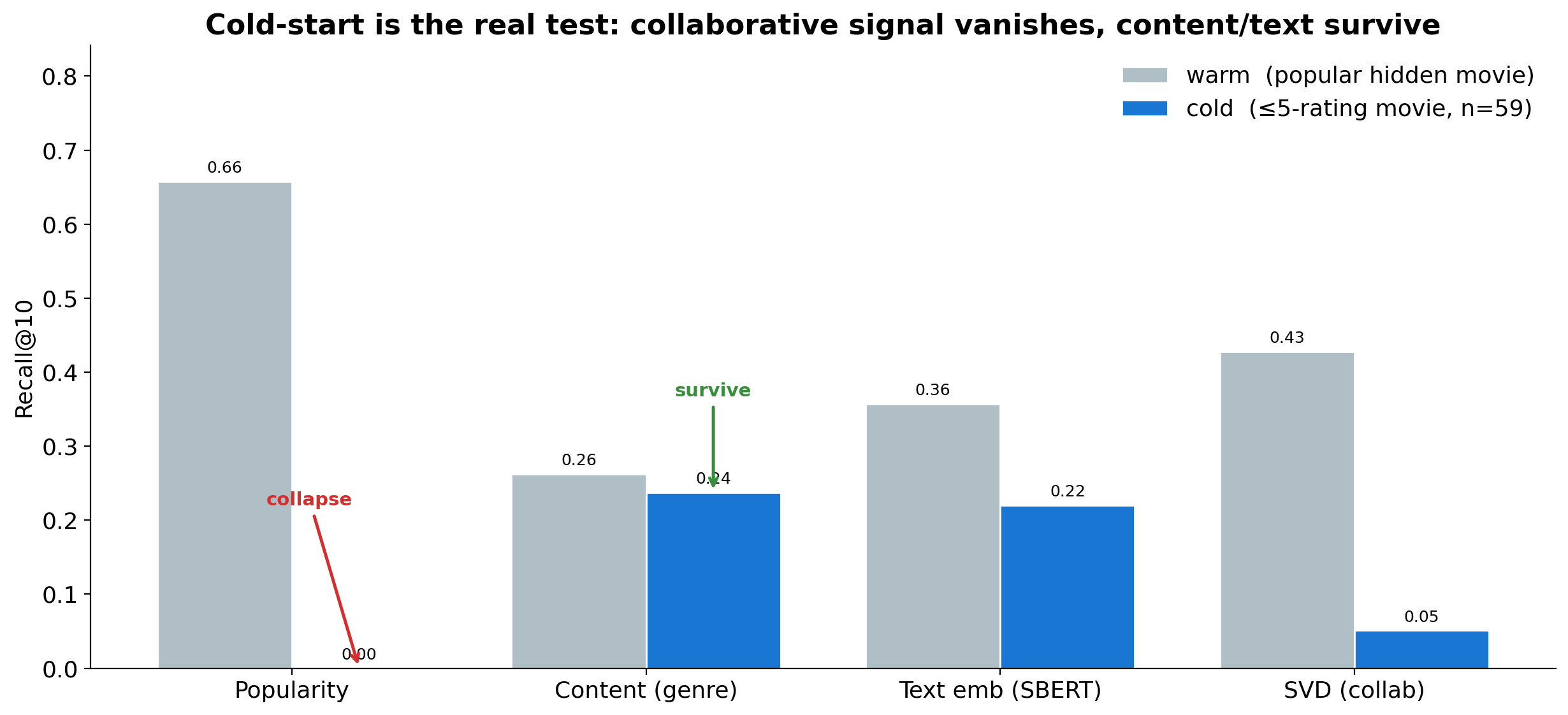
Collaborative signal needs a substantial interaction history; with ≤5 ratings the learned item factor is missing or far too noisy to rank — so SVD collapses. A feature-based embedding (genres, text — and, with posters, images) still places the item from its content alone. This is the payoff of the whole arc: content embeddings are what make cold-start tractable — and exactly why we built the multimodal image tower.
Evaluating your project — you supply the ground truth
Awareness
— appreciate the idea, don’t memorize the internals.
For your final project you’ll evaluate your own retrieval system. Our MovieLens eval borrowed labels from user behavior (we hid a rating) — but your dataset may have no user log at all, just items (repos, papers, products…).
So you must supply the relevance judgments — for each query, which items count as correct answers (the IR shorthand for this is qrels, short for query relevance judgments). Then the same metrics apply (Recall@k · NDCG@k · MRR).
Two ways to build these relevance judgments for your data:
(1) Self-supervised pairs — free: a docstring is a query for its code, a README for its repo. Each is one known-relevant item → a whole test set at no cost.
(2) Human annotation — write queries and label what’s relevant by hand (next slide).
Source
# Three routes to relevance judgments (qrels) when there is no user log -> the SAME retrieval metrics.
fig, ax = plt.subplots(figsize=(13.5, 5.8)); ax.axis('off')
ax.set_xlim(0, 15); ax.set_ylim(0, 8)

def _gb(cx, cy, w, h, t, fc, ec, fs=10.5, tc='white'):
    ax.add_patch(FancyBboxPatch((cx - w/2, cy - h/2), w, h, boxstyle='round,pad=0.04',
                                facecolor=fc, edgecolor=ec, lw=2))
    ax.text(cx, cy, t, ha='center', va='center', fontsize=fs, fontweight='bold', color=tc)

def _ga(x0, y0, x1, y1, col='#555'):
    ax.annotate('', xy=(x1, y1), xytext=(x0, y0), arrowprops=dict(arrowstyle='-|>', color=col, lw=2.2))

# top: the TWO routes that build qrels for YOUR data -> qrels -> the same metrics
srcs = [('Self-supervised pairs\n(docstring → code, README → repo)', GREEN,  6.0),
        ('Human annotation\n(Label Studio, Session 1)',              ORANGE, 4.3)]
for t, col, y in srcs:
    _gb(2.9, y, 4.0, 1.2, t, col, 'white', 9.4)
    _ga(4.95, y, 6.45, 5.15, col)
_gb(8.05, 5.15, 3.0, 1.5, 'relevance judgments\n(correct items for\nYOUR queries)', '#37474f', '#263238', 9.5)
_ga(9.6, 5.15, 10.95, 5.15)
_gb(12.85, 5.15, 3.4, 1.5, 'Recall@k · NDCG@k\nMRR', '#fffde7', '#fbc02d', 10, '#333')
ax.text(8.05, 6.6, 'ground truth for YOUR data', ha='center', fontsize=10.5, color=GREEN, fontweight='bold')

# bottom (separate, dashed): a public benchmark tests the ENCODER on its OWN data — not your items
ax.add_patch(FancyBboxPatch((1.0, 0.6), 13.2, 1.95, boxstyle='round,pad=0.04',
                            fill=False, edgecolor=BLUE, lw=2, linestyle='--'))
ax.text(7.6, 2.05, 'SEPARATE — a public benchmark (BEIR · MTEB · CodeSearchNet)',
        ha='center', fontsize=10.5, color=BLUE, fontweight='bold')
ax.text(7.6, 1.2, 'ships its OWN queries + relevance judgments → checks whether your ENCODER is a good retriever in general\n'
        '(it does not evaluate your system on your items)', ha='center', fontsize=9.3, color='#333')

ax.set_title('Two ways to build ground truth for YOUR items → the same retrieval metrics', fontweight='bold')
plt.tight_layout(); plt.show()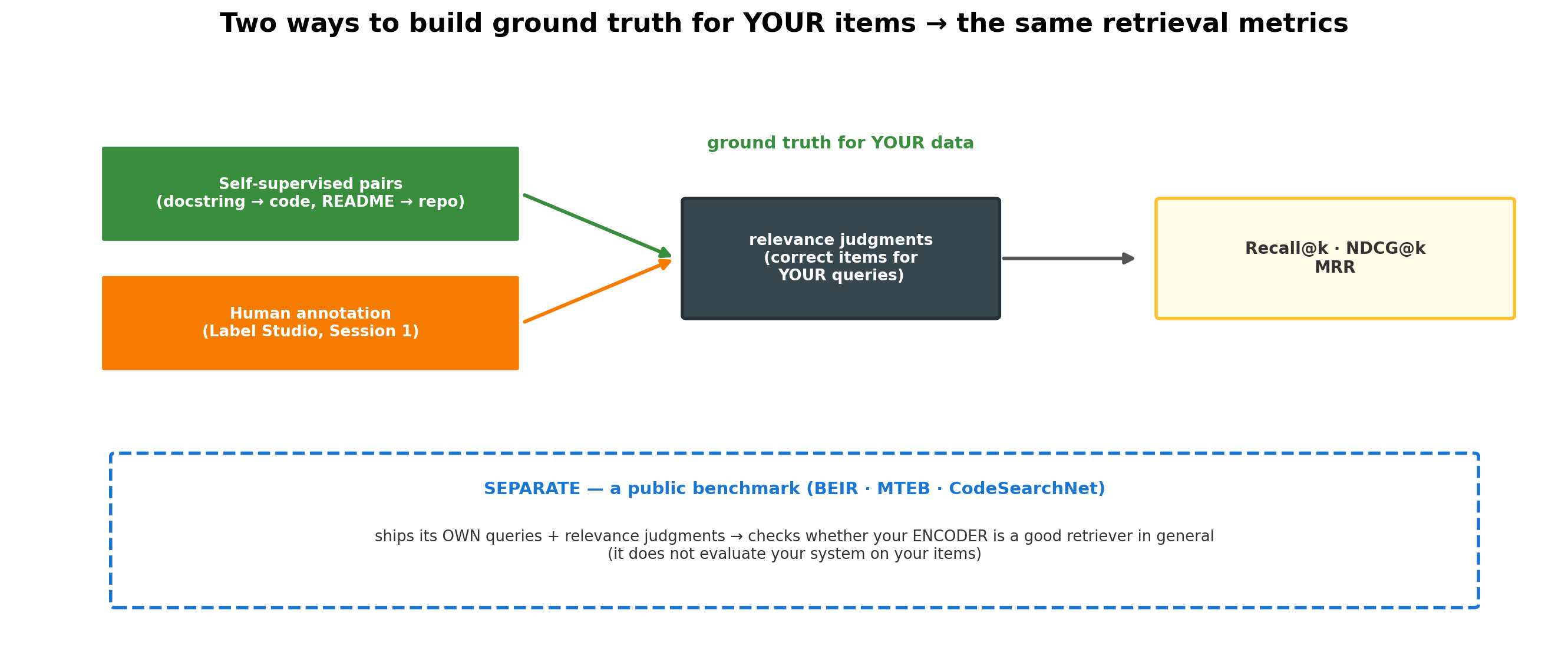
A public benchmark is a different tool (slide after next): it ships its own queries + relevance judgments, so it tests whether your encoder is a good retriever in general — not your system on your items. MRR (Mean Reciprocal Rank), in one sentence: if the first correct hit sits at rank r the query scores (rank 1 → 1.0, rank 2 → 0.5, …), averaged over all queries.
Building relevance judgments by hand (Label Studio)
Awareness
— appreciate the idea, don’t memorize the internals.
When no natural pairs exist (or you want real relevance): write ~30–50 representative queries, retrieve candidates, and label each (query, item) relevant / not — graded 0–3 if you want NDCG.
This is exactly the Label Studio pipeline from Session 1 (Data Acquisition) — same tool, now labeling (query, document) pairs instead of raw records.
Pooling keeps it affordable: judge only the top-k of a few systems, treat everything unjudged as not-relevant.
Use ≥2 annotators and report inter-annotator agreement (Cohen’s / Fleiss’ κ, also from Session 1): if humans can’t agree on what’s relevant, the metric is just noise. And the labels, though gold, are incomplete — an unjudged-but-relevant item is scored as a miss (the same missing-not-at-random caveat from the last slide).
Public benchmarks — sanity-check the encoder
Awareness
— appreciate the idea, don’t memorize the internals.
A different question: not “is my system good on my data?” but “is my encoder a good retriever at all?” Run it on a benchmark that already ships queries + relevance judgments — match the task shape to your project:
text retrieval → BEIR (zero-shot, 18 datasets), MTEB (the embedding leaderboard), MS MARCO, Natural Questions
code search → CodeSearchNet, CoIR
image ↔ text → MS COCO · Flickr30K (caption↔image retrieval), ImageNet (CLIP zero-shot), MMEB / MIEB (multimodal leaderboards)
The pipeline is a few lines (it downloads the data, so run it offline — not in this notebook):
import mteb
from sentence_transformers import SentenceTransformer

model = SentenceTransformer("all-MiniLM-L6-v2")        # your encoder (a CLIP model for image↔text)
tasks = mteb.get_tasks(tasks=["SciFact", "NFCorpus"])  # pick benchmark tasks by name
results = mteb.MTEB(tasks=tasks).run(model)            # downloads, embeds, scores → NDCG@10 · Recall@k · MRR
A benchmark tests the encoder on its data, not your system on your items — so report a public-benchmark number and a small hand-labeled set from your own data. MTEB / BEIR are also where you’d pick which pretrained encoder to start from.
Wrap-up: everything became a vector — in one space
The whole course, in one line:
S6 framed the problem — sparsity, the long tail, cold-start.
S7 → S9 turned genres → ratings → text into vectors (content-based, matrix factorization, neural embeddings).
S10, today: images joined them — a movie’s plot, its poster, and its audience now all live in one shared space.
The one idea under all of it: every method turns users and items into vectors in one shared space and ranks them by a dot product — whether that vector comes from a trained encoder (text, images), a learned lookup (SVD, autoencoder), or simply averaging item features (content). One evaluation harness then scores them all head-to-head.
Once both sides are vectors, recommending and searching run on the same machinery — nearest-neighbour retrieval — even though the questions they answer differ.
One honest caveat to take with you: offline metrics are only a proxy (ratings are missing-not-at-random — people rate what they were shown), so the real test is online — clicks, dwell time, A/B tests.
- Cremonesi, P., Koren, Y., & Turrin, R. (2010). Performance of recommender algorithms on top-n recommendation tasks. Proceedings of the Fourth ACM Conference on Recommender Systems, 39–46. 10.1145/1864708.1864721