Session 8: Matrix Factorization & Learned Embeddings
“Last week we hand-built the vectors. Today the model learns them — and we prove they’re good.”
Core idea: stop hand-crafting features. Decompose the rating matrix so that every user and every item becomes a learned vector in one shared space — an embedding.
Source
# Setup — run this first
import importlib.util, subprocess, sys
_need = {'pandas': 'pandas', 'numpy': 'numpy', 'matplotlib': 'matplotlib',
         'seaborn': 'seaborn', 'scikit-learn': 'sklearn', 'torch': 'torch',
         'scikit-surprise': 'surprise'}
_missing = [pip for pip, mod in _need.items() if importlib.util.find_spec(mod) is None]
if _missing:
    subprocess.run([sys.executable, '-m', 'pip', 'install', '-q', *_missing], check=False)

import pandas as pd
import numpy as np
import matplotlib.pyplot as plt
import seaborn as sns
from sklearn.decomposition import PCA
from sklearn.metrics.pairwise import cosine_similarity
from sklearn.metrics import roc_curve, roc_auc_score
from sklearn.model_selection import train_test_split
import urllib.request, zipfile, os

plt.rcParams.update({'figure.figsize': (12, 6), 'font.size': 13, 'axes.titlesize': 16})
np.random.seed(42)

# MovieLens (small) — downloaded at runtime, not committed
if not os.path.exists('ml-latest-small'):
    urllib.request.urlretrieve(
        'https://files.grouplens.org/datasets/movielens/ml-latest-small.zip', 'ml.zip')
    with zipfile.ZipFile('ml.zip', 'r') as z:
        z.extractall('.')

ratings = pd.read_csv('ml-latest-small/ratings.csv')
movies = pd.read_csv('ml-latest-small/movies.csv')

# consecutive integer ids for matrix rows/cols
user_ids = ratings['userId'].unique()
movie_ids = ratings['movieId'].unique()
user_to_idx = {u: i for i, u in enumerate(user_ids)}
movie_to_idx = {m: i for i, m in enumerate(movie_ids)}
idx_to_movie = {i: m for m, i in movie_to_idx.items()}
n_users, n_movies = len(user_ids), len(movie_ids)
ratings['user_idx'] = ratings['userId'].map(user_to_idx)
ratings['movie_idx'] = ratings['movieId'].map(movie_to_idx)

# dense rating matrix R (missing entries = 0)
R = np.zeros((n_users, n_movies))
for row in ratings.itertuples():
    R[row.user_idx, row.movie_idx] = row.rating

# one fixed train/test split reused everywhere (SVD/SGD/ALS/eval)
train, test = train_test_split(ratings, test_size=0.2, random_state=42)
tr_u, tr_i, tr_r = train['user_idx'].values, train['movie_idx'].values, train['rating'].values
te_u, te_i, te_r = test['user_idx'].values, test['movie_idx'].values, test['rating'].values

print(f'{n_users} users x {n_movies} movies, {len(ratings):,} ratings '
      f'({100*len(ratings)/(n_users*n_movies):.2f}% filled)')
610 users x 9724 movies, 100,836 ratings (1.70% filled)
Recap: content-based filtering (Session 7)
Describe each item by its features (genre columns), build a user profile from what they liked, rank by cosine similarity.
✅ No other users needed — works day one, handles new items.
⚠️ Stuck with hand-crafted features; every “Drama” gets the identical vector.
Today’s learned vectors fix that.
Source
# Content-based recap (Session 7): items as genre vectors, ranked by cosine similarity.
rc_genres = ['Action', 'SciFi', 'Romance', 'Drama', 'Comedy']
rc_titles = ['Star Wars', 'The Matrix', 'Titanic', 'The Notebook']
rc_M = np.array([[1, 1, 0, 0, 0],
                 [1, 1, 0, 0, 0],
                 [0, 0, 1, 1, 0],
                 [0, 0, 1, 1, 0]], dtype=float)
rc_sim = cosine_similarity(rc_M)[0]              # similarity of every film to Star Wars (row 0)
fig, (axA, axB) = plt.subplots(1, 2, figsize=(14, 4.5), gridspec_kw={'width_ratios': [3, 2]})
sns.heatmap(rc_M, annot=True, fmt='.0f', cmap='Greys', vmin=0, vmax=1.4, cbar=False,
            linewidths=1, linecolor='white', xticklabels=rc_genres, yticklabels=rc_titles, ax=axA)
axA.set_yticklabels(rc_titles, rotation=0, va='center')
axA.set_xticklabels(rc_genres, rotation=45, ha='right')
axA.set_title('Movies as genre vectors', fontweight='bold')
axB.barh(range(4), rc_sim, color=['#1976d2', '#388e3c', '#d32f2f', '#f57c00'])
axB.set_yticks(range(4)); axB.set_yticklabels(rc_titles); axB.invert_yaxis()
axB.set_xlim(0, 1.05); axB.set_xlabel('cosine similarity to Star Wars')
axB.set_title('Rank by similarity to a liked film', fontweight='bold')
for i, v in enumerate(rc_sim):
    axB.text(v + 0.02, i, f'{v:.2f}', va='center', fontweight='bold')
axB.spines[['top', 'right']].set_visible(False)
plt.tight_layout()
plt.show()
print('Content-based needs no other users — but it only sees the features we hand-craft.')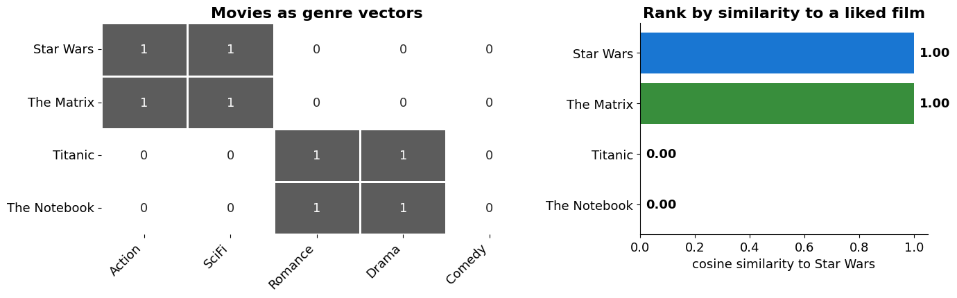
Content-based needs no other users — but it only sees the features we hand-craft.
Recap: collaborative filtering
Forget item features — collaborative filtering predicts from the crowd, using only the user × item rating matrix and people who behaved like you.
User-based: find users who rated like you, borrow their opinions.
Item-based: find items rated alike, recommend the neighbours.
“Birds of a feather flock together.” Today we make it model-based — learn from that matrix instead of looking up neighbours each query.
Source
# Collaborative filtering recap: predict from similar USERS — no item features used.
rc_R = np.array([[5, 4, 5, 1, 2],
                 [4, 5, 4, 2, 1],          # B — rates like E
                 [1, 2, 1, 5, 4],
                 [5, 4, 4, 1, 2],          # D — rates like E
                 [4, 5, np.nan, 1, 2]], dtype=float)  # E -> item 3 = ?
rc_users = ['A', 'B', 'C', 'D', 'E']
rc_items = [f'item {j}' for j in range(1, 6)]
from matplotlib.colors import ListedColormap
WHITE = ListedColormap(['white'])
fig, ax = plt.subplots(figsize=(9, 4.5))
sns.heatmap(rc_R, mask=np.isnan(rc_R), annot=True, fmt='.0f', cmap=WHITE, cbar=False,
            linewidths=1.5, linecolor='#cccccc', annot_kws={'fontsize': 13, 'color': 'black'},
            xticklabels=rc_items, yticklabels=rc_users, ax=ax)
ax.set_yticklabels(rc_users, rotation=0, va='center')
for sp in ax.spines.values():
    sp.set_visible(True); sp.set_color('#888')
ax.add_patch(plt.Rectangle((2, 4), 1, 1, fill=False, edgecolor='#7b1fa2', lw=4))   # the "?"
ax.text(2.5, 4.5, '?', ha='center', va='center', fontsize=22, fontweight='bold', color='#7b1fa2')
for r in (1, 3):                                                                   # look-alike users
    ax.add_patch(plt.Rectangle((0, r), 5, 1, fill=False, edgecolor='#388e3c', lw=3))
ax.set_title("Collaborative filtering: E's ? is filled from look-alike users B & D", fontweight='bold')
plt.tight_layout()
plt.show()
print('CF uses only the rating matrix — who rated similarly — never the movie content.')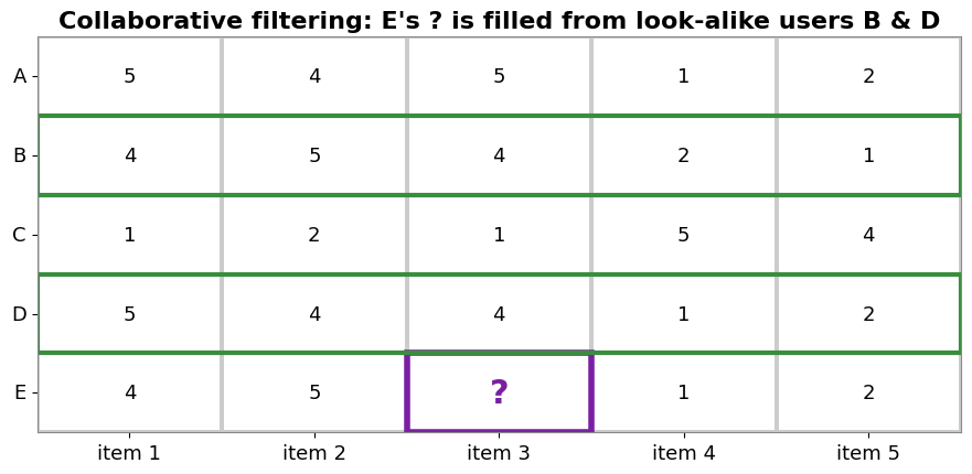
CF uses only the rating matrix — who rated similarly — never the movie content.
A quick look: Bayes for binary ratings
Treat a missing cell as classification: will user D like item 2 (+1) or not (−1)? Use the ratings we do have, via Bayes’ rule:
Interpretable, and it works — but it returns a probability for one cell. Run it for every item and you just refill D’s row of — never a reusable vector to cluster or search. That’s what today fixes.
Source
# Illustrative ±1 like/dislike matrix — predict the "?" cell from the others.
from matplotlib.colors import ListedColormap
WHITE = ListedColormap(['white'])
fig, (axL, axR) = plt.subplots(1, 2, figsize=(15, 5), gridspec_kw={'width_ratios': [3, 2]})

R_toy = np.array([
    [ 1,  1, -1, np.nan, np.nan, np.nan],
    [ 1,  1, np.nan, np.nan, np.nan,  1],
    [np.nan, np.nan, np.nan,  1, -1, -1],
    [-1, np.nan,  1, np.nan, np.nan, np.nan],
], dtype=float)
target = (3, 1)  # user D, item 2 -> the "?"

sns.heatmap(R_toy, mask=np.isnan(R_toy), annot=True, fmt='.0f', cmap=WHITE,
            cbar=False, linewidths=1.5, linecolor='#cccccc', annot_kws={'fontsize': 14, 'color': 'black'},
            xticklabels=[f'item {j}' for j in range(1, 7)],
            yticklabels=['A', 'B', 'C', 'D'], ax=axL)
for sp in axL.spines.values():
    sp.set_visible(True); sp.set_color('#888')
axL.add_patch(plt.Rectangle((target[1], target[0]), 1, 1, fill=False, edgecolor='#7b1fa2', lw=4))
axL.text(target[1] + 0.5, target[0] + 0.5, '?', ha='center', va='center',
         fontsize=26, fontweight='bold', color='#7b1fa2')
axL.set_title('Will user D like item 2?  (+1 / −1)', fontweight='bold')

# illustrative posterior from Bayes' rule on the other cells
axR.bar(['P(+1)\nlikes', 'P(−1)\ndislikes'], [0.72, 0.28],
        color=['#388e3c', '#d32f2f'], edgecolor='white', width=0.6)
axR.set_ylim(0, 1)
axR.axhline(0.5, color='gray', ls='--', lw=1)
for x, v in zip([0, 1], [0.72, 0.28]):
    axR.text(x, v + 0.02, f'{v:.2f}', ha='center', fontsize=14, fontweight='bold')
axR.set_title('Bayes gives a probability…\n…but no reusable latent vector for D', fontweight='bold')
axR.spines[['top', 'right']].set_visible(False)
plt.tight_layout()
plt.show()
print('Predicting one cell at a time is fine — but it never produces a reusable representation.')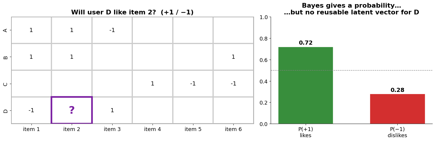
Predicting one cell at a time is fine — but it never produces a reusable representation.
Recap: how do we measure a recommender? ROC & AUROC
Call an item relevant if the user rated it ≥ 4. A model outputs a score per item; sweep a threshold and trace true-positive rate vs false-positive rate → the ROC curve.
0.5 = coin flip (the diagonal) · 1.0 = perfect ranking.
One number to compare any two methods — here a dumb popularity baseline already clears chance.
(AUROC scores ranking. Today we predict the actual rating value, so the final scoreboard uses RMSE — average prediction error — instead. Same idea: one number, lower is better.)
Source
# Real ROC on our held-out test set. Baseline score = how popular the movie is.
test_label = (te_r >= 4).astype(int)               # relevant = rating >= 4

pop = np.zeros(n_movies)                            # popularity = #ratings per movie (train)
counts = train.groupby('movie_idx').size()
pop[counts.index.values] = counts.values
score_pop = pop[te_i]

fpr, tpr, _ = roc_curve(test_label, score_pop)
auc_pop = roc_auc_score(test_label, score_pop)

fig, ax = plt.subplots(figsize=(7.5, 7))
ax.plot(fpr, tpr, color='#1976d2', lw=3, label=f'Popularity baseline (AUROC = {auc_pop:.3f})')
ax.plot([0, 1], [0, 1], color='gray', ls='--', lw=1.5, label='coin flip (AUROC = 0.5)')
ax.fill_between(fpr, tpr, alpha=0.12, color='#1976d2')
ax.set_xlabel('False-positive rate')
ax.set_ylabel('True-positive rate')
ax.set_title('ROC — popularity baseline (the bar to beat)', fontweight='bold')
ax.legend(loc='lower right', fontsize=11)
ax.spines[['top', 'right']].set_visible(False)
plt.tight_layout()
plt.show()
print(f'Popularity already beats chance ({auc_pop:.3f}) — popular movies tend to be rated higher.')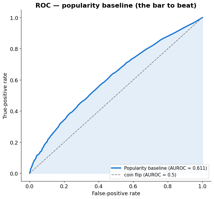
Popularity already beats chance (0.611) — popular movies tend to be rated higher.
Today: from predicting cells to learning vectors
Bayes showed road 1 of model-based CF: predict one missing cell from . It works — but hands back a number, no reusable vector. There’s a second road:
Predict the cell directly — Bayes · kNN. A number, no vector. (just saw it)
Learn a vector per user & item — SVD, gradient descent, autoencoders → embeddings. ← today
Road 2 lets the model discover the structure in and hands us vectors we can reuse, search, transfer.
Source
# Roadmap: the two branches of model-based collaborative filtering.
fig, ax = plt.subplots(figsize=(13, 5.5))
ax.set_xlim(0, 1); ax.set_ylim(0, 1); ax.axis('off')

def box(x, y, w, h, text, fc, ec, fs=12, fw='normal'):
    ax.add_patch(plt.Rectangle((x, y), w, h, facecolor=fc, edgecolor=ec, lw=2, zorder=2))
    ax.text(x + w / 2, y + h / 2, text, ha='center', va='center',
            fontsize=fs, fontweight=fw, zorder=3)

box(0.02, 0.40, 0.20, 0.20, 'Rating matrix $R$\n(mostly empty)', '#fff9c4', '#f9a825', 13, 'bold')

# branch A — predict directly
box(0.38, 0.66, 0.26, 0.16, 'Predict the cell directly\nBayes · kNN', '#ffebee', '#d32f2f', 12)
box(0.74, 0.66, 0.24, 0.16, 'a number\nno reusable vector', '#fafafa', '#bbb', 11, 'bold')
# branch B — learn vectors
box(0.38, 0.16, 0.26, 0.16, 'Learn a vector per\nuser & item\nSVD · SGD/ALS · Autoencoder', '#e3f2fd', '#1976d2', 12)
box(0.74, 0.16, 0.24, 0.16, 'EMBEDDINGS\nshared vector space', '#e8f5e9', '#388e3c', 12, 'bold')

for (x0, y0, x1, y1, c) in [(0.22, 0.50, 0.38, 0.74, '#d32f2f'),
                            (0.22, 0.50, 0.38, 0.24, '#1976d2'),
                            (0.64, 0.74, 0.74, 0.74, '#999'),
                            (0.64, 0.24, 0.74, 0.24, '#388e3c')]:
    ax.annotate('', xy=(x1, y1), xytext=(x0, y0),
                arrowprops=dict(arrowstyle='->', color=c, lw=2.2))
ax.text(0.86, 0.60, '↑ we just did this (Bayes)', ha='center', fontsize=11,
        color='#d32f2f', fontweight='bold')
ax.text(0.86, 0.10, '↑ today we take this road', ha='center', fontsize=12,
        color='#388e3c', fontweight='bold')
ax.set_title('Model-based collaborative filtering: predict a number, or learn a vector?',
             fontweight='bold')
plt.tight_layout()
plt.show()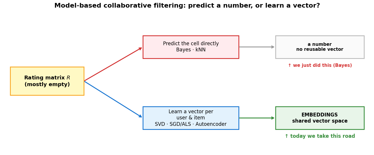
First, the key idea: dimension reduction
A movie described by all its genres is long and redundant — sci-fi/action/adventure/fantasy move together; romance/drama/musical/family too. Those columns really live on a few underlying axes.
That’s : the number of hidden factors we keep. Squeeze a high-dimensional, correlated description down to coordinates that carry the signal — users get the same treatment, in the same space.
Source
# Dimension reduction: many correlated genres collapse to k hidden factors.
# (local names are dr_-prefixed so we don't clobber the global `movies` DataFrame)
fig, axes = plt.subplots(1, 3, figsize=(15, 4.2),
                         gridspec_kw={'width_ratios': [4, 0.6, 1.6]})
dr_movies = ['SW', 'Matrix', 'Titanic', 'Notebk', 'P&P']
dr_genres = ['SciFi', 'Action', 'Advent', 'Fantasy', 'Romance', 'Drama', 'Musical', 'Family']

# high-dimensional genre indicator: first 4 genres cluster, last 4 cluster
dr_G = np.array([[1, 1, 1, 1, 0, 0, 0, 0],   # SW       -> action/sci-fi cluster
                 [1, 1, 1, 0, 0, 0, 0, 0],   # Matrix   -> action/sci-fi cluster
                 [0, 0, 0, 0, 1, 1, 0, 1],   # Titanic  -> romance/drama cluster
                 [0, 0, 0, 0, 1, 1, 1, 0],   # Notebook -> romance/drama cluster
                 [0, 0, 0, 0, 1, 1, 1, 1]], dtype=float)  # P&P
sns.heatmap(dr_G, annot=True, fmt='.0f', cmap='Greys', vmin=0, vmax=1.4, cbar=False, ax=axes[0],
            linewidths=1, linecolor='white', xticklabels=dr_genres, yticklabels=dr_movies)
axes[0].set_title('Movies × 8 genres  (high-dim, redundant)', fontweight='bold', fontsize=13)
axes[0].set_xticklabels(dr_genres, rotation=45, ha='right')  # genres angled so they don't collide
axes[0].set_yticklabels(dr_movies, rotation=0, va='center')  # movie names horizontal & readable

axes[1].text(0.5, 0.5, 'reduce\n$\\rightarrow$', fontsize=20, ha='center', va='center',
             fontweight='bold', color='#7b1fa2'); axes[1].axis('off')

# the same movies, now in k = 2 latent coordinates (foreshadows Q)
dr_F = np.array([[0.9, 0.1], [0.8, 0.1], [0.1, 0.9], [0.1, 0.85], [0.05, 0.95]])
sns.heatmap(dr_F, annot=True, fmt='.2f', cmap='Greens', cbar=False, ax=axes[2],
            linewidths=1, linecolor='white', xticklabels=['f₁', 'f₂'], yticklabels=dr_movies)
axes[2].set_title('Movies × k = 2 factors', fontweight='bold', fontsize=13)
axes[2].set_yticklabels(dr_movies, rotation=0, va='center')
plt.suptitle('Dimension reduction: 8 correlated genres → k = 2 hidden axes',
             fontsize=15, fontweight='bold', y=1.04)
plt.tight_layout()
plt.show()
print('f₁ ≈ "action/sci-fi", f₂ ≈ "romance/drama". k = how many axes we keep — that is the whole point of k.')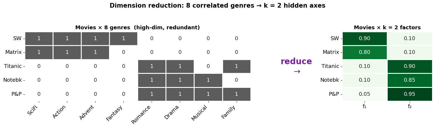
f₁ ≈ "action/sci-fi", f₂ ≈ "romance/drama". k = how many axes we keep — that is the whole point of k.
The leap: one shared latent space
The Bayes/kNN road builds a fresh predictor for each user from that user’s own row — nothing is shared, nothing is reused. Instead, learn one vector per user and one vector per item in the same -dimensional space, so that
= user factors ( users × ) · = item factors ( items × ), with .
A hidden factor might mean “action-vs-romance”, “blockbuster-vs-arthouse” — but the model discovers them.
Source
# What matrix factorization looks like: R  ≈  P × Qᵀ
from matplotlib.colors import ListedColormap
WHITE = ListedColormap(['white'])
fig, axes = plt.subplots(1, 5, figsize=(16, 4),
                         gridspec_kw={'width_ratios': [4, 0.5, 2, 0.5, 2]})
R_ex = np.array([[5, 3, np.nan, 1, np.nan],
                 [4, np.nan, np.nan, 1, np.nan],
                 [np.nan, 1, 5, 4, 4],
                 [np.nan, np.nan, 4, 5, np.nan]])
sns.heatmap(R_ex, mask=np.isnan(R_ex), annot=True, fmt='.0f', cmap=WHITE, cbar=False, ax=axes[0],
            linewidths=1, linecolor='#cccccc', annot_kws={'color': 'black'},
            xticklabels=['SW', 'Matrix', 'Titanic', 'Notebk', 'P&P'],
            yticklabels=['Alice', 'Bob', 'Carol', 'Dave'])
for sp in axes[0].spines.values():
    sp.set_visible(True); sp.set_color('#888')
axes[0].set_title('R  (ratings, with holes)', fontweight='bold', fontsize=13)
axes[1].text(0.5, 0.5, '≈', fontsize=30, ha='center', va='center', fontweight='bold'); axes[1].axis('off')
P_ex = np.array([[0.9, 0.1], [0.8, 0.2], [0.1, 0.9], [0.2, 0.8]])
sns.heatmap(P_ex, annot=True, fmt='.1f', cmap='Blues', cbar=False, ax=axes[2],
            linewidths=1, linecolor='white', xticklabels=['f₁', 'f₂'],
            yticklabels=['Alice', 'Bob', 'Carol', 'Dave'])
axes[2].set_title('P  (user factors)', fontweight='bold', fontsize=13)
axes[3].text(0.5, 0.5, '×', fontsize=30, ha='center', va='center', fontweight='bold'); axes[3].axis('off')
Q_ex = np.array([[0.9, 0.7, 0.1, 0.1, 0.0], [0.1, 0.2, 0.9, 0.8, 0.9]])
sns.heatmap(Q_ex, annot=True, fmt='.1f', cmap='Greens', cbar=False, ax=axes[4],
            linewidths=1, linecolor='white',
            xticklabels=['SW', 'Matrix', 'Titanic', 'Notebk', 'P&P'], yticklabels=['f₁', 'f₂'])
axes[4].set_title('Qᵀ  (item factors)', fontweight='bold', fontsize=13)
plt.suptitle('Matrix Factorization:  R ≈ P × Qᵀ   (illustrative factors; k = 2 hidden factors)',
             fontsize=15, fontweight='bold', y=1.05)
plt.tight_layout()
plt.show()
print('Illustrative taste-weights in [0,1]: their dot products reproduce the high→low PATTERN of the '
      'ratings (e.g. Alice·SW = 0.82 high, Alice·Titanic = 0.18 low). The exact factors come from SVD next.')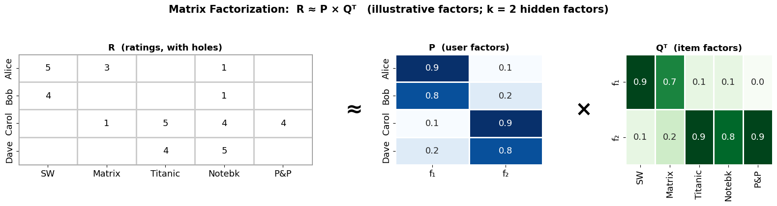
Illustrative taste-weights in [0,1]: their dot products reproduce the high→low PATTERN of the ratings (e.g. Alice·SW = 0.82 high, Alice·Titanic = 0.18 low). The exact factors come from SVD next.
SVD, geometrically: every matrix is rotate → stretch → rotate
A matrix times a vector is a linear transformation — it moves points around space. Remarkable fact: any linear map, however messy, is just a rotation, then a stretch along the axes, then another rotation (more precisely, are orthogonal — rotation, possibly with a reflection). SVD writes exactly that:
The stretch factors are the singular values — how much each new axis is stretched = how much signal that direction carries.
Source
# rotate (Vᵀ) -> stretch (Σ) -> rotate (U). Track the right-singular vectors v1, v2 (the principal axes).
M = np.array([[2.0, 1.0], [0.5, 1.5]])
Ug, sg, Vtg = np.linalg.svd(M)
V = Vtg.T
v1, v2 = V[:, 0:1], V[:, 1:2]                     # input principal directions (orthonormal)
th = np.linspace(0, 2 * np.pi, 200)
circle = np.vstack([np.cos(th), np.sin(th)])
stages = [('1. unit circle', np.eye(2)),
          (r'2. after $V^T$ (rotate)', Vtg),
          (r'3. after $\Sigma V^T$ (stretch)', np.diag(sg) @ Vtg),
          (r'4. after $U\Sigma V^T = M$ (rotate)', Ug @ np.diag(sg) @ Vtg)]

fig, axes = plt.subplots(1, 5, figsize=(20, 4.4))
for ax, (t, T) in zip(axes[:4], stages):
    pts = T @ circle
    ax.plot(pts[0], pts[1], color='#1976d2', lw=2)
    for vec, c in [(T @ v1, '#d32f2f'), (T @ v2, '#388e3c')]:   # singular vectors stay on the ellipse axes
        ax.annotate('', xy=(vec[0, 0], vec[1, 0]), xytext=(0, 0),
                    arrowprops=dict(arrowstyle='->', color=c, lw=2.5))
    ax.set_title(t, fontweight='bold', fontsize=11)

axc = axes[4]                                      # the same map applied in ONE step, for comparison
axc.plot(circle[0], circle[1], color='#9e9e9e', lw=1.5, ls='--', label='start: circle')
ell = M @ circle
axc.plot(ell[0], ell[1], color='#1976d2', lw=2, label='end: ellipse')
for vec, c in [(v1, '#d32f2f'), (v2, '#388e3c')]:
    axc.annotate('', xy=(vec[0, 0], vec[1, 0]), xytext=(0, 0),
                 arrowprops=dict(arrowstyle='->', color=c, lw=1.5, ls='--', alpha=0.55))
for vec, c in [(M @ v1, '#d32f2f'), (M @ v2, '#388e3c')]:
    axc.annotate('', xy=(vec[0, 0], vec[1, 0]), xytext=(0, 0),
                 arrowprops=dict(arrowstyle='->', color=c, lw=2.5))
axc.set_title(r'$M$ in one step (compare with 4)', fontweight='bold', fontsize=11)
axc.legend(fontsize=8, loc='lower right')

for ax in axes:
    ax.set_xlim(-3, 3); ax.set_ylim(-3, 3); ax.set_aspect('equal'); ax.grid(alpha=0.2)
    ax.axhline(0, color='gray', lw=0.5); ax.axvline(0, color='gray', lw=0.5)
plt.suptitle(rf'$M = U\Sigma V^T$,  $\sigma = ({sg[0]:.2f},\ {sg[1]:.2f})$   —   '
             r'red/green = right-singular vectors $v_1, v_2$', fontsize=13, fontweight='bold')
plt.tight_layout()
plt.show()
print('Σ stretches along the singular axes: |Mv₁|=σ₁, |Mv₂|=σ₂ — the arrows ARE the ellipse axes.')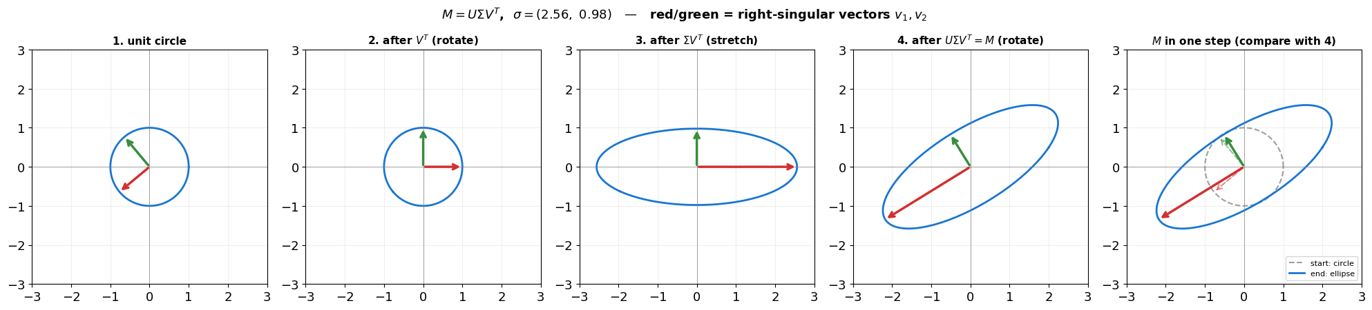
Σ stretches along the singular axes: |Mv₁|=σ₁, |Mv₂|=σ₂ — the arrows ARE the ellipse axes.
Where do U, Σ, V come from? (it’s PCA, twice)
You met PCA: find the orthogonal directions of greatest variance — the eigenvectors of the covariance matrix. SVD is PCA run on both sides of at once:
= eigenvectors of → the item–item matrix (which items co-vary)
= eigenvectors of → the user–user matrix (which users co-vary)
→ the signal strength of each shared direction (largest first)
Both sides share the same axes — that is why users and items land in one space.
(Strictly, is the covariance only once is mean-centred; on raw ratings it’s the uncentered scatter matrix — same eigenvectors idea. We subtract the mean a couple of slides on.)
Source
# Each matrix -> its eigenvectors. RRᵀ gives U (users), RᵀR gives V (items). No colour: the numbers matter.
from matplotlib.colors import ListedColormap
WHITE = ListedColormap(['white'])
Rm = np.array([[5, 5, 4, 2, 1, 1], [5, 5, 5, 1, 1, 2],
               [2, 1, 1, 4, 4, 3], [1, 1, 2, 5, 5, 4]], float)
U2, s2, Vt2 = np.linalg.svd(Rm, full_matrices=False)
user_cov, item_cov, V = Rm @ Rm.T, Rm.T @ Rm, Vt2.T
fac = [r'$\alpha$', r'$\beta$', r'$\gamma$', r'$\delta$']   # the 4 latent-factor axes

def _table(ax, M, fmt, xt, yt):                  # plain gridded matrix
    sns.heatmap(M, annot=True, fmt=fmt, cmap=WHITE, cbar=False, linewidths=1, linecolor='#cccccc',
                annot_kws={'color': 'black'}, xticklabels=xt, yticklabels=yt, ax=ax)
    ax.set_yticklabels(yt, rotation=0)
    for s in ax.spines.values():
        s.set_visible(True); s.set_color('#888'); s.set_linewidth(1.2)

def _vectors(ax, M, xt, yt):                      # columns separated by bold lines = orthogonal unit vectors
    sns.heatmap(M, annot=True, fmt='.2f', cmap=WHITE, cbar=False, linewidths=0,
                annot_kws={'color': 'black'}, xticklabels=xt, yticklabels=yt, ax=ax)
    ax.set_yticklabels(yt, rotation=0)
    for x in range(M.shape[1] + 1):
        ax.axvline(x, color='black', lw=2)
    ax.axhline(0, color='black', lw=2); ax.axhline(M.shape[0], color='black', lw=2)

fig = plt.figure(figsize=(15, 9))
gs = fig.add_gridspec(2, 3, width_ratios=[1.05, 0.62, 0.95])
aUL, aUR = fig.add_subplot(gs[0, 0]), fig.add_subplot(gs[0, 2])
aLL, aLR = fig.add_subplot(gs[1, 0]), fig.add_subplot(gs[1, 2])
ac = fig.add_subplot(gs[:, 1]); ac.axis('off'); ac.set_xlim(0, 1); ac.set_ylim(0, 1)
_table(aUL, user_cov, '.0f', list('ABCD'), list('ABCD')); aUL.set_title(r'user–user  $R R^T$', fontweight='bold')
_vectors(aUR, U2, fac, list('ABCD')); aUR.set_title(r'$U$  (columns = user vectors)', fontweight='bold')
_table(aLL, item_cov, '.0f', range(1, 7), range(1, 7)); aLL.set_title(r'item–item  $R^T R$', fontweight='bold')
_vectors(aLR, V, fac, range(1, 7)); aLR.set_title(r'$V$  (columns = item vectors)', fontweight='bold')
# arrows  RRᵀ -> U  and  RᵀR -> V , with the σ link sitting between the four matrices
for y in (0.78, 0.22):
    ac.annotate('', xy=(0.95, y), xytext=(0.05, y), arrowprops=dict(arrowstyle='-|>', color='#333', lw=2.5))
    ac.text(0.5, y + 0.08, 'eigenvectors', ha='center', fontsize=11, fontweight='bold', color='#333')
ac.text(0.5, 0.54, r'$\sigma_k=\sqrt{\lambda_k}$', ha='center', va='center', fontsize=14, fontweight='bold')
ac.text(0.5, 0.45, rf'$\sigma=({s2[0]:.2f},\,{s2[1]:.2f},$' + '\n' + rf'${s2[2]:.2f},\,{s2[3]:.2f})$',
        ha='center', va='center', fontsize=11,
        bbox=dict(boxstyle='round,pad=0.3', fc='#fff8e1', ec='#f9a825'))
fig.suptitle(r'$U$ = eigenvectors of $RR^T$,  $V$ = eigenvectors of $R^TR$  (every column is a unit vector)',
             fontsize=14, fontweight='bold')
plt.tight_layout()
plt.show()
print('Columns are unit length:  ‖U cols‖ =', np.linalg.norm(U2, axis=0).round(2),
      ' and orthonormal (UᵀU = I):', np.allclose(U2.T @ U2, np.eye(4)))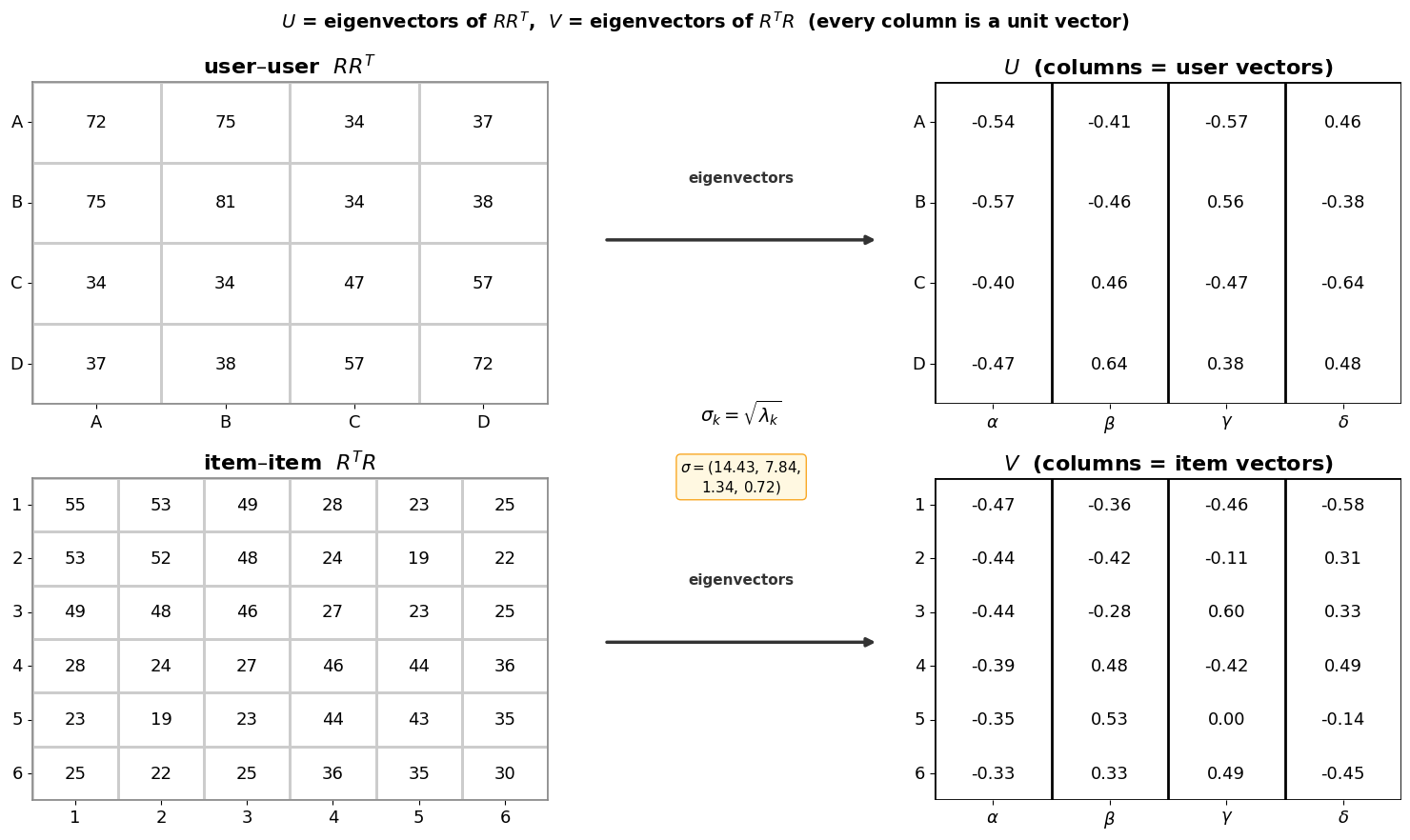
Columns are unit length: ‖U cols‖ = [1. 1. 1. 1.] and orthonormal (UᵀU = I): True
A full example: decompose, then drop the weak axes
Our toy (4 users × 6 items) has two clear groups — A,B love items 1–3, C,D love 4–6 — so its SVD has two big singular values and two tiny ones. Keep the top 2 triplets → the best rank-2 approximation (Eckart–Young): a faithful at small Frobenius error .
🧠 Same trick today: LoRA fine-tunes huge LLMs by freezing the big weight matrix and learning only a small low-rank update — the same “big matrix ≈ two skinny ones” idea.
Source
# Full SVD as matrices: R = U Σ Vᵀ. Keep the 2 biggest singular triplets (red) -> R ≈ R₂.
from matplotlib.colors import ListedColormap
WHITE = ListedColormap(['white'])
Rm = np.array([[5, 5, 4, 2, 1, 1], [5, 5, 5, 1, 1, 2],
               [2, 1, 1, 4, 4, 3], [1, 1, 2, 5, 5, 4]], float)   # two clear groups -> near rank 2
U2, s2, Vt2 = np.linalg.svd(Rm, full_matrices=False)
S = np.diag(s2)
R2 = U2[:, :2] @ np.diag(s2[:2]) @ Vt2[:2, :]
GR = [r'$\alpha$', r'$\beta$', r'$\gamma$', r'$\delta$']

def _grid(ax, M, fmt, xt, yt, title, ann=None):
    sns.heatmap(M, annot=(ann if ann is not None else True), fmt=('' if ann is not None else fmt),
                cmap=WHITE, cbar=False, linewidths=1, linecolor='#cccccc',
                annot_kws={'color': 'black', 'fontsize': 10}, xticklabels=xt, yticklabels=yt, ax=ax)
    ax.set_yticklabels(yt, rotation=0)
    for sp in ax.spines.values():
        sp.set_visible(True); sp.set_color('#888'); sp.set_linewidth(1.2)
    ax.set_title(title, fontweight='bold', fontsize=11)

def _hl(ax, x, y, w, h):                          # red box = the kept top-2 factors
    ax.add_patch(plt.Rectangle((x, y), w, h, fill=False, edgecolor='#d32f2f', lw=3, zorder=5))

fig = plt.figure(figsize=(17, 8.5))
top, bot = fig.subfigures(2, 1, height_ratios=[1.05, 1])
aR, sep1, aU, sep2, aS, sep3, aVt = top.subplots(1, 7, gridspec_kw={'width_ratios': [6, 0.5, 4, 0.5, 4, 0.5, 6]})
for sx in (sep1, sep2, sep3):
    sx.axis('off')
sep1.text(0.5, 0.5, '=', ha='center', va='center', fontsize=26, fontweight='bold')
sep2.text(0.5, 0.5, r'$\cdot$', ha='center', va='center', fontsize=30, fontweight='bold')
sep3.text(0.5, 0.5, r'$\cdot$', ha='center', va='center', fontsize=30, fontweight='bold')
_grid(aR, Rm, '.0f', range(1, 7), list('ABCD'), r'$R$  (ratings)')
_grid(aU, U2, '.2f', GR, list('ABCD'), r'$U$')
Sann = [[f'{S[i, j]:.2f}' if i == j else '' for j in range(4)] for i in range(4)]
_grid(aS, S, '.2f', GR, GR, r'$\Sigma$', ann=Sann)
_grid(aVt, Vt2, '.2f', range(1, 7), GR, r'$V^T$')
_hl(aU, 0, 0, 2, 4); _hl(aS, 0, 0, 2, 2); _hl(aVt, 0, 0, 6, 2)
top.subplots_adjust(top=0.78)                     # breathing room under the title
top.suptitle(r'Full SVD:  $R = U\,\Sigma\,V^T$.    $\sigma_1$ and $\sigma_2$ have by far the largest effect (red).',
             fontweight='bold', fontsize=14, y=0.99)

aR2, sc, aRo = bot.subplots(1, 3, gridspec_kw={'width_ratios': [6, 1.3, 6]})
sc.axis('off')
sc.text(0.5, 0.6, r'$\approx$', ha='center', va='center', fontsize=30, fontweight='bold')
sc.text(0.5, 0.33, f'Frobenius\n‖R−R₂‖ = {np.sqrt(np.sum((Rm - R2)**2)):.2f}', ha='center', va='center',
        fontsize=11, color='#d32f2f', fontweight='bold')
_grid(aR2, R2, '.1f', range(1, 7), list('ABCD'), r'$R_2 = U_2\,\Sigma_2\,V_2^T$  (only the top-2 factors)')
_grid(aRo, Rm, '.0f', range(1, 7), list('ABCD'), r'$R$  (original)')
bot.subplots_adjust(top=0.86)
plt.show()
print(f'σ = {s2.round(2)}.  Keep σ₁,σ₂=({s2[0]:.1f},{s2[1]:.1f}), drop σ₃,σ₄=({s2[2]:.1f},{s2[3]:.1f}) '
      f'→ R₂ rebuilds R with error {np.sqrt(np.sum((Rm - R2)**2)):.2f}.')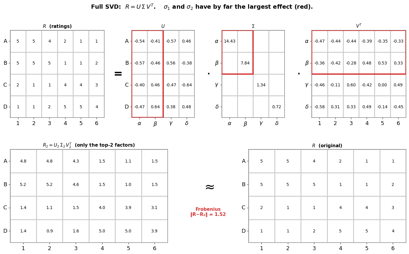
σ = [14.43 7.84 1.34 0.72]. Keep σ₁,σ₂=(14.4,7.8), drop σ₃,σ₄=(1.3,0.7) → R₂ rebuilds R with error 1.52.
From three matrices to two: 
Fold in — absorb the stretch into the two sides:
Every user is a row of , every item a column of — short vectors in one shared -dim space: the embeddings. One rating = one dot product.
( is the standard recommender notation. Folding in means is no longer orthonormal.)
Source
# P = UΣ (users), Qᵀ = Vᵀ (items), R = P·Qᵀ. Read a rating as: user ROW of P · item COLUMN of Qᵀ.
from matplotlib.colors import ListedColormap
WHITE = ListedColormap(['white'])
Rm = np.array([[5, 5, 4, 2, 1, 1], [5, 5, 5, 1, 1, 2],
               [2, 1, 1, 4, 4, 3], [1, 1, 2, 5, 5, 4]], float)
U2, s2, Vt2 = np.linalg.svd(Rm, full_matrices=False)
kk = 2
Pf = U2[:, :kk] * s2[:kk]                          # (4 x 2) user factors = U·Σ  (a row per user)
Qf = Vt2[:kk, :]                                   # (2 x 6) item factors = Vᵀ   (a row per eigenvector)
Rhat = Pf @ Qf                                     # (4 x 6) reconstruction P·Qᵀ

def _grid(ax, M, fmt, xt, yt, title, vsep=False, hsep=False, redbox=None):
    sns.heatmap(M, annot=True, fmt=fmt, cmap=WHITE, cbar=False, linewidths=1, linecolor='#dddddd',
                annot_kws={'color': 'black'}, xticklabels=xt, yticklabels=yt, ax=ax)
    ax.set_yticklabels(yt, rotation=0)
    for sp in ax.spines.values():
        sp.set_visible(True); sp.set_color('#888'); sp.set_linewidth(1.2)
    if vsep:                                       # bold dividers between COLUMNS
        for x in range(M.shape[1] + 1): ax.axvline(x, color='black', lw=2)
    if hsep:                                       # bold dividers between ROWS
        for y in range(M.shape[0] + 1): ax.axhline(y, color='black', lw=2)
    if redbox:
        ax.add_patch(plt.Rectangle(redbox[:2], redbox[2], redbox[3], fill=False, edgecolor='#d32f2f', lw=3, zorder=6))
    ax.set_title(title, fontweight='bold', fontsize=12)

fig, (a1, sp1, a2, sp2, a3) = plt.subplots(1, 5, figsize=(18, 4),
        gridspec_kw={'width_ratios': [1.3, 0.3, 3.0, 0.3, 3.0]})
sp1.axis('off'); sp1.text(0.5, 0.5, '×', ha='center', va='center', fontsize=26, fontweight='bold')
sp2.axis('off'); sp2.text(0.5, 0.5, '=', ha='center', va='center', fontsize=26, fontweight='bold')
# P: each ROW is one user; the two COLUMNS are the user-side latent axes -> vertical dividers
_grid(a1, Pf, '.2f', [r'$\alpha$', r'$\beta$'], list('ABCD'),
      r'$P=U\Sigma$  (each row = one user)', vsep=True, redbox=(0, 0, 2, 1))
# Qᵀ: each ROW is one eigenvector (right-singular vector); each COLUMN is one item -> horizontal dividers
_grid(a2, Qf, '.2f', [f'item{j}' for j in range(1, 7)], [r'$\alpha$', r'$\beta$'],
      r'$Q^T=V^T$  (each ROW = one eigenvector, each col = one item)', hsep=True, redbox=(0, 0, 1, 2))
_grid(a3, Rhat, '.1f', [f'item{j}' for j in range(1, 7)], list('ABCD'),
      r'$R = P\,Q^{T}$  (every rating reconstructed)', redbox=(0, 0, 1, 1))
pred = Pf[0] @ Qf[:, 0]
plt.suptitle(rf'$\hat r_{{A,1}}=\vec p_A\cdot\vec q_1={pred:.2f}$  (actual {Rm[0, 0]:.0f})  —  a ROW of $P$ times a COLUMN of $Q^T$',
             fontsize=14, fontweight='bold', y=1.05)
plt.tight_layout()
plt.show()
print('Three matrices became two. Row A of P · column 1 of Qᵀ = the (A,1) entry of R = P·Qᵀ.')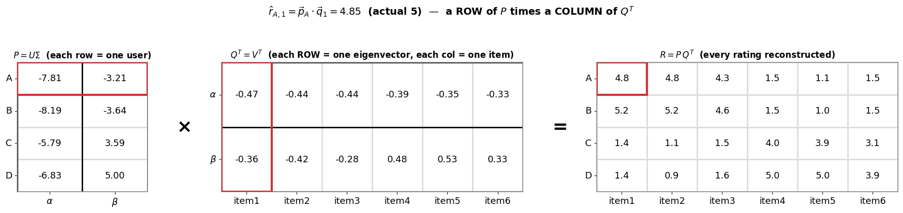
Three matrices became two. Row A of P · column 1 of Qᵀ = the (A,1) entry of R = P·Qᵀ.
The catch: SVD needs a full matrix
Real rating matrices are mostly empty, and plain SVD has no notion of “missing”. The textbook hack: set every unknown to 0 — but 0 means “hated it”, not “unseen”, so the factorization bends to fit millions of fake zeros.
The fix: fit only the observed cells, plus regularization to stop the few ratings overfitting:
( = global average, subtracted first.) No closed form → Gradient Descent or ALS.
Source
# Plain SVD has no "missing": the classic hack sets every unknown rating to 0. But 0 means "hated it"!
from matplotlib.colors import ListedColormap
WHITE = ListedColormap(['white'])
R_sparse = np.array([[5, 0, 4, 0, 0, 1],
                     [0, 5, 0, 0, 2, 0],
                     [4, 0, 0, 5, 0, 0],
                     [0, 1, 0, 4, 0, 5],
                     [0, 0, 5, 0, 1, 0]], float)
obs = R_sparse > 0
its, us = [f'i{j}' for j in range(1, 7)], list('ABCDE')

def _grid(ax, draw_zeros, title):                 # plain numbers on a white grid — no value colouring
    sns.heatmap(np.zeros_like(R_sparse), cmap=WHITE, cbar=False, linewidths=1.5, linecolor='#cccccc',
                xticklabels=its, yticklabels=us, ax=ax)
    ax.set_yticklabels(us, rotation=0)
    for sp in ax.spines.values():
        sp.set_visible(True); sp.set_color('#888')
    for i in range(R_sparse.shape[0]):
        for j in range(R_sparse.shape[1]):
            if obs[i, j]:
                ax.text(j + 0.5, i + 0.5, f'{int(R_sparse[i, j])}', ha='center', va='center', fontsize=12)
            elif draw_zeros:
                ax.text(j + 0.5, i + 0.5, '0', ha='center', va='center',
                        color='#d32f2f', fontweight='bold', fontsize=13)
    ax.set_title(title, fontweight='bold')

fig, (b1, b2) = plt.subplots(1, 2, figsize=(14, 4.8))
_grid(b1, False, 'What we actually know  (blank = unrated)')
_grid(b2, True, 'What SVD is fed: unknown → 0  (red 0 = fabricated)')
plt.suptitle('"Fill the holes with 0" — but 0 means "hated it", not "unrated"', fontweight='bold', y=1.02)
plt.tight_layout()
plt.show()
print(f'{int((~obs).sum())} of {obs.size} cells were unknown — all silently turned into "0 stars".')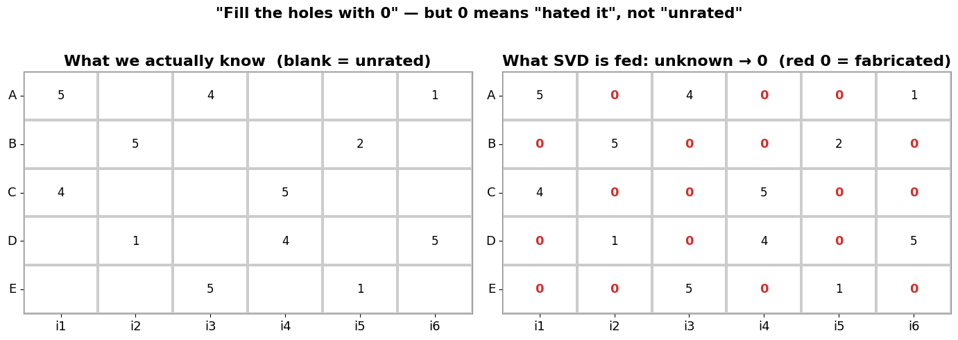
18 of 30 cells were unknown — all silently turned into "0 stars".
How do we minimize it? Gradient descent
No closed form anymore — so roll downhill. For a function , repeatedly step against the slope:
is the learning rate. A steep slope → a big step; at the bottom the slope is 0 and we stop.
Source
# Gradient descent on f(x) = (x-1)^2 + 5  — a 1-D warm-up.
f  = lambda x: (x - 1)**2 + 5
df = lambda x: 2 * x - 2                          # f'(x) = 2x - 2
x, alpha, path = 10.0, 0.1, [10.0]
for _ in range(25):
    x = x - alpha * df(x)                         # the learning step
    path.append(x)
path = np.array(path)

fig, (a1, a2) = plt.subplots(1, 2, figsize=(14, 4.8))
xs = np.linspace(-9, 11, 200)
a1.plot(xs, f(xs), color='#1976d2', lw=2)
x0 = path[2]; slope = df(x0)                      # the gradient = slope of the tangent here
tx = np.linspace(x0 - 3, x0 + 3, 2)
a1.plot(tx, f(x0) + slope * (tx - x0), color='#f57c00', lw=2.5, ls='--', zorder=2,
        label="tangent = gradient $f'(x)$")       # the ONE gradient line
a1.plot(path, f(path), 'o', color='#d32f2f', ms=6, zorder=4, label='GD steps')  # markers only — no second line
a1.annotate(f"slope = f '(x) = {slope:.0f}\n(the gradient)", (x0, f(x0)), xytext=(5.6, 98), ha='left',
            fontsize=10, fontweight='bold', color='#f57c00', arrowprops=dict(arrowstyle='->', color='#f57c00'))
a1.scatter([1], [f(1)], color='#388e3c', s=120, zorder=5, label='minimum x=1')
a1.set_title(r"step against the slope: $x \leftarrow x - \alpha\,f'(x)$", fontweight='bold')
a1.set_xlabel('x'); a1.set_ylabel('f(x)'); a1.legend(loc='upper left'); a1.spines[['top', 'right']].set_visible(False)
a2.plot(path, 'o-', color='#d32f2f')
a2.axhline(1, ls='--', color='#388e3c', label='target x=1')
a2.set_title('x converges to the minimum', fontweight='bold')
a2.set_xlabel('iteration'); a2.legend(); a2.spines[['top', 'right']].set_visible(False)
plt.tight_layout()
plt.show()
print(f'Started at x=10; after 25 steps x={path[-1]:.3f} (true minimum 1), learning rate α={alpha}.')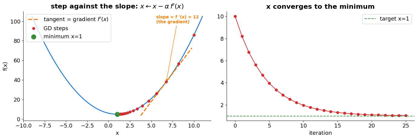
Started at x=10; after 25 steps x=1.034 (true minimum 1), learning rate α=0.1.
The same recipe, applied to our loss
For one observed rating (taking as already mean-centred):
① error ② loss
③ slope — each factor gets its own gradient (chain rule):
④ step downhill (fold the 2 into ):
Under-predicted ()? Nudge toward , by the error. The keeps vectors small (no overfit).
Source
# One GD step moves BOTH factors at once: -∂J/∂p nudges the user vector, -∂J/∂q nudges the item vector.
r, lam, alpha = 4.0, 0.1, 0.05
p0, q0 = 0.8, 1.2
e = r - p0 * q0
gp = -2 * e * q0 + 2 * lam * p0                  # ∂J/∂p  (the user-factor gradient)
gq = -2 * e * p0 + 2 * lam * q0                  # ∂J/∂q  (the item-factor gradient)
ng = np.array([-gp, -gq]); L = 1.25 * ng / np.linalg.norm(ng)   # downhill direction, fixed length for drawing

fig, ax = plt.subplots(figsize=(7.6, 6))
P, Q = np.meshgrid(np.linspace(-0.3, 4.5, 250), np.linspace(-0.3, 4.5, 250))
ax.contourf(P, Q, (r - P * Q)**2 + lam * (P**2 + Q**2), levels=np.linspace(0, 40, 25), cmap='YlGnBu', extend='max')
ax.annotate('', xy=(p0 + L[0], q0), xytext=(p0, q0), arrowprops=dict(arrowstyle='-|>', color='#d32f2f', lw=3))
ax.annotate('', xy=(p0 + L[0], q0 + L[1]), xytext=(p0 + L[0], q0), arrowprops=dict(arrowstyle='-|>', color='#388e3c', lw=3))
ax.annotate('', xy=(p0 + L[0], q0 + L[1]), xytext=(p0, q0), arrowprops=dict(arrowstyle='-|>', color='black', lw=2, ls=':'))
ax.plot(p0, q0, 'o', color='black', ms=11, zorder=6)
ax.text(p0 + L[0] / 2, q0 - 0.28, r'$-\partial J/\partial p$', color='#d32f2f', fontweight='bold', ha='center', fontsize=13)
ax.text(p0 + L[0] / 2, q0 - 0.6, 'update USER factor', color='#d32f2f', fontweight='bold', ha='center', fontsize=10)
ax.text(p0 + L[0] + 0.12, q0 + L[1] / 2, r'$-\partial J/\partial q$', color='#388e3c', fontweight='bold', va='center', fontsize=13)
ax.text(p0 + L[0] + 0.12, q0 + L[1] / 2 - 0.32, 'update ITEM factor', color='#388e3c', fontweight='bold', va='center', fontsize=10)
ax.text(p0 + L[0] / 2 - 0.2, q0 + L[1] / 2 + 0.2, 'gradient step', color='black', fontsize=10, rotation=20)
ax.set_xlim(-0.3, 4.5); ax.set_ylim(-0.3, 4.5)
ax.set_xlabel('p  (user factor)'); ax.set_ylabel('q  (item factor)')
ax.set_title('One gradient step moves BOTH factors\n'
             r'$p\leftarrow p+\alpha(e\,q-\lambda p)$,   $q\leftarrow q+\alpha(e\,p-\lambda q)$',
             fontweight='bold', fontsize=12)
plt.tight_layout()
plt.show()
print(f'At (p,q)=({p0},{q0}): error e={e:.2f}. The downhill step has a p-part (user) AND a q-part (item) — both update together.')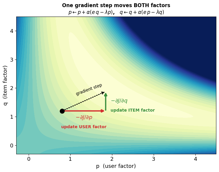
At (p,q)=(0.8,1.2): error e=3.04. The downhill step has a p-part (user) AND a q-part (item) — both update together.
Source
# Same update, swept: ONE rating r=4, ONE latent dim (k=1). GD rolls down the real loss surface.
r, lam, alpha = 4.0, 0.1, 0.05
Lf = lambda p, q: (r - p * q)**2 + lam * (p**2 + q**2)
p, q = 0.8, 1.2                                  # a (bad) starting guess
path = [(p, q)]
for _ in range(15):                              # ~5 steps already nail it — no need for 60
    e = r - p * q                                # ① error
    p = p + alpha * (e * q - lam * p)            # ④ the update rule — user factor
    q = q + alpha * (e * p - lam * q)            # ④ the update rule — item factor
    path.append((p, q))
path = np.array(path)

fig, (a1, a2) = plt.subplots(1, 2, figsize=(14, 5.2))
P, Q = np.meshgrid(np.linspace(-0.3, 4.5, 250), np.linspace(-0.3, 4.5, 250))
a1.contourf(P, Q, (r - P * Q)**2 + lam * (P**2 + Q**2), levels=np.linspace(0, 40, 25),
            cmap='YlGnBu', extend='max')
a1.plot(path[:, 0], path[:, 1], 'o-', color='#d32f2f', ms=6, lw=1.8, mec='black', mew=0.6, zorder=4)
a1.plot(*path[0], 'o', color='black', ms=12, label='start', zorder=6)
a1.plot(*path[8], 's', color='#ffeb3b', ms=13, mec='black', label='step 8 (already good)', zorder=6)
a1.plot(*path[-1], '*', color='#ff5252', ms=20, mec='black', mew=0.6, label='converged', zorder=6)
a1.set_xlabel('p  (user factor)'); a1.set_ylabel('q  (item factor)')
a1.set_title(r'loss $L(p,q)=(4-pq)^2+\lambda(p^2{+}q^2)$ — GD rolls downhill', fontweight='bold', fontsize=12)
a1.legend(loc='upper right')
losses = [Lf(pp, qq) for pp, qq in path]
a2.plot(losses, 'o-', color='#1976d2', lw=2, ms=5)
a2.axvline(8, ls='--', color='#388e3c')
a2.text(8.3, max(losses) * 0.72, 'flat by step ~8', color='#388e3c', fontweight='bold')
a2.set_title('loss falls fast — essentially flat after ~7–8 steps', fontweight='bold')
a2.set_xlabel('iteration'); a2.set_ylabel('L'); a2.spines[['top', 'right']].set_visible(False)
plt.tight_layout()
plt.show()
print(f'p·q = {path[8,0]*path[8,1]:.2f} by step 8, {path[-1,0]*path[-1,1]:.2f} at the end ≈ r = 4 '
      f'(slightly below 4 because the λ penalty keeps the vectors small).')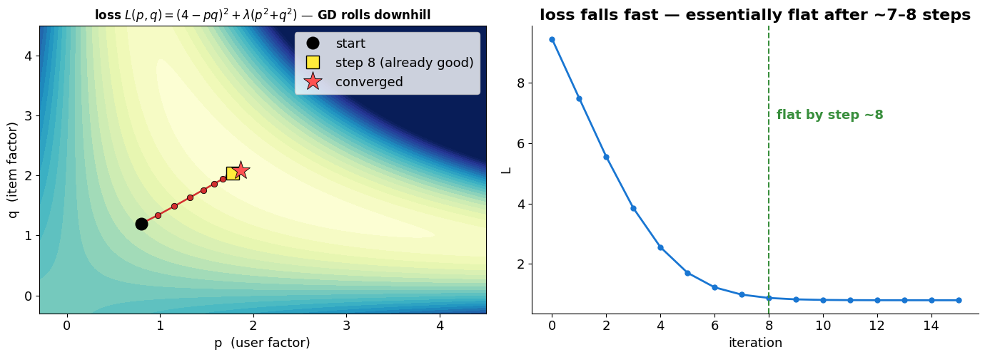
p·q = 3.62 by step 8, 3.89 at the end ≈ r = 4 (slightly below 4 because the λ penalty keeps the vectors small).
Putting it together: fill the whole sparse matrix
The same update, swept over every observed cell, factorises a real matrix with holes. Start from random ; gradient-descend on the observed ratings only; then read off :
learn — random → after sweeps matches on the knowns;
predict , rounded to — knowns reproduced, holes filled.
Source
# Learn P, Q by GD on the OBSERVED cells only. random init -> after n iterations P·Qᵀ matches R.
from matplotlib.colors import ListedColormap
WHITE = ListedColormap(['white'])
R_obs = np.array([[5, 3, np.nan, 1, np.nan, 5],
                  [4, np.nan, np.nan, 1, 1, np.nan],
                  [1, 1, np.nan, 5, np.nan, 2],
                  [np.nan, 1, 5, 4, np.nan, np.nan]], float)
obs = ~np.isnan(R_obs)
m, n, kk = 4, 6, 2
rng = np.random.default_rng(0)
P, Q = rng.random((m, kk)), rng.random((n, kk))   # P: user factors (m×k), Q: item factors (n×k)
P_init, Q_init = P.copy(), Q.copy()               # snapshot the random start
init_pred = P @ Q.T
for step in range(4000):                          # the SAME per-cell update, swept to convergence
    for i in range(m):
        for j in range(n):
            if obs[i, j]:
                e = R_obs[i, j] - P[i] @ Q[j]
                P[i] += 0.02 * (e * Q[j] - 0.05 * P[i])
                Q[j] += 0.02 * (e * P[i] - 0.05 * Q[j])
fin_pred = P @ Q.T

def _tab(ax, M, fmt, xt, yt, title, cmap=WHITE, mask=None, center=None, vmin=None, vmax=None):
    sns.heatmap(M, annot=True, fmt=fmt, cmap=cmap, cbar=False, linewidths=1, linecolor='#cccccc',
                annot_kws={'color': 'black', 'fontsize': 10}, xticklabels=xt, yticklabels=yt, ax=ax,
                mask=mask, center=center, vmin=vmin, vmax=vmax)
    ax.set_yticklabels(yt, rotation=0); ax.set_title(title, fontweight='bold', fontsize=10)

fig, axes = plt.subplots(2, 4, figsize=(18, 7), gridspec_kw={'width_ratios': [1.1, 2.6, 2.6, 2.6]})
items = [f'it{j}' for j in range(1, 7)]; usr = list('ABCD'); fac = [r'$\alpha$', r'$\beta$']
_tab(axes[0, 0], P_init, '.2f', fac, usr, r'$P$  (random)')
_tab(axes[0, 1], Q_init.T, '.2f', items, fac, r'$Q^T$  (random)')
_tab(axes[0, 2], init_pred, '.1f', items, usr, r'$P Q^T$  (random → garbage)')
_tab(axes[0, 3], R_obs, '.0f', items, usr, r'$R$  (observed only)', mask=~obs)
_tab(axes[1, 0], P, '.2f', fac, usr, r'$P$  (after $n$)')
_tab(axes[1, 1], Q.T, '.2f', items, fac, r'$Q^T$  (after $n$)')
_tab(axes[1, 2], fin_pred, '.1f', items, usr, r'$P Q^T$  (after $n$ ≈ R)')
_tab(axes[1, 3], R_obs, '.0f', items, usr, r'$R$  (observed only)', mask=~obs)
plt.suptitle('Learn $P,Q$ by gradient descent on the OBSERVED cells: random init → after $n$ iterations $P Q^T$ matches $R$',
             fontweight='bold', y=1.02)
plt.tight_layout()
plt.show()
print(f'RMSE on the observed cells after 4000 sweeps: {np.sqrt(np.mean((R_obs[obs] - fin_pred[obs])**2)):.3f}.')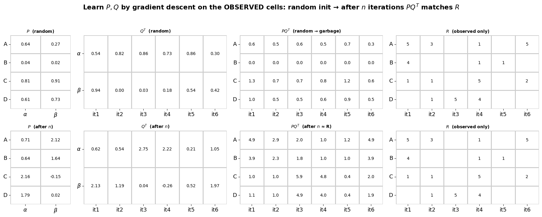
RMSE on the observed cells after 4000 sweeps: 0.070.
Source
# Reconstruct R̂ = P Qᵀ, round to 1-5. green = matches a known, yellow = newly filled hole.
from matplotlib.patches import Patch
fin_pred = P @ Q.T                                # reuse the P, Q learned in the previous cell
pred_round = np.clip(np.rint(fin_pred), 1, 5).astype(int)
items = [f'it{j}' for j in range(1, 7)]; usr = list('ABCD')
GREEN, YELLOW, RED = '#a5d6a7', '#fff59d', '#ef9a9a'

fig, ax = plt.subplots(figsize=(11, 4.6))
for i in range(R_obs.shape[0]):
    for j in range(R_obs.shape[1]):
        col = YELLOW if not obs[i, j] else (GREEN if pred_round[i, j] == int(R_obs[i, j]) else RED)
        ax.add_patch(plt.Rectangle((j, R_obs.shape[0] - 1 - i), 1, 1, facecolor=col, edgecolor='#999', lw=1.2))
        ax.text(j + 0.5, R_obs.shape[0] - 1 - i + 0.5, str(pred_round[i, j]),
                ha='center', va='center', fontweight='bold', fontsize=14)
ax.set_xlim(0, R_obs.shape[1]); ax.set_ylim(0, R_obs.shape[0]); ax.set_aspect('equal')
ax.set_xticks([j + 0.5 for j in range(R_obs.shape[1])]); ax.set_xticklabels(items)
ax.set_yticks([R_obs.shape[0] - 1 - i + 0.5 for i in range(R_obs.shape[0])]); ax.set_yticklabels(usr)
ax.tick_params(length=0)
for sp in ax.spines.values():
    sp.set_visible(False)
ax.legend(handles=[Patch(facecolor=GREEN, edgecolor='#999', label='correct (= a known rating)'),
                   Patch(facecolor=YELLOW, edgecolor='#999', label='new prediction (was a hole)'),
                   Patch(facecolor=RED, edgecolor='#999', label='wrong')],
          loc='upper left', bbox_to_anchor=(1.01, 1.0), frameon=False)
ax.set_title(r'$\hat R = P Q^T$ rounded to 1–5: knowns reproduced (green), holes filled (yellow)',
             fontweight='bold')
plt.tight_layout()
plt.show()
filled = int((~obs).sum())
print(f'Every one of the {filled} empty cells now has a 1–5 prediction — the recommender can rank them.')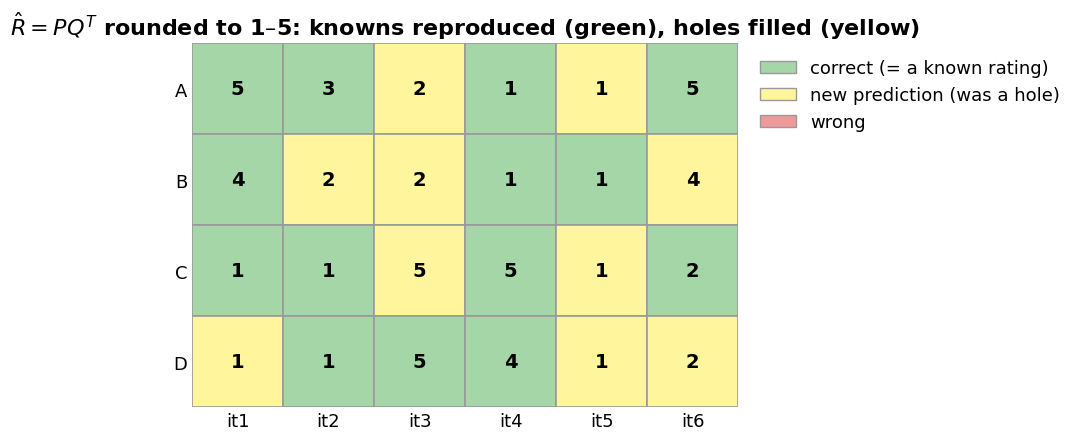
Every one of the 10 empty cells now has a 1–5 prediction — the recommender can rank them.
The other optimizer: Alternating Least Squares (ALS)
Gradient descent takes thousands of tiny steps. ALS is the shortcut: the loss is hard in and together, but fix one and it’s an ordinary least-squares problem in the other.
Hold fixed → solving each user’s is ridge regression — one exact closed-form solve.
Then hold fixed → solve every . Repeat.
Each step is exact, so it converges in a handful of alternations, and every user (and item) solves
independently → embarrassingly parallel. That’s why ALS is the workhorse for huge implicit-feedback
datasets (Spark MLlib, implicit).
Source
# ALS on the same toy: fix Q → solve P, fix P → solve Q. Same goal as GD, in a few exact steps.
R_obs = np.array([[5, 3, np.nan, 1, np.nan, 5],
                  [4, np.nan, np.nan, 1, 1, np.nan],
                  [1, 1, np.nan, 5, np.nan, 2],
                  [np.nan, 1, 5, 4, np.nan, np.nan]], float)
obs = ~np.isnan(R_obs)
m, n, kk, lam = 4, 6, 2, 0.1
rng = np.random.default_rng(1)
P, Q, Ik = rng.random((m, kk)), rng.random((n, kk)), np.eye(kk)
errs = []
for it in range(6):
    for i in range(m):                                 # fix Q, solve each user row p_i by ridge LSQ
        j = obs[i]
        if j.any():
            Qj = Q[j]; P[i] = np.linalg.solve(Qj.T @ Qj + lam * Ik, Qj.T @ R_obs[i, j])
    for j in range(n):                                 # fix P, solve each item column q_j
        i = obs[:, j]
        if i.any():
            Pi = P[i]; Q[j] = np.linalg.solve(Pi.T @ Pi + lam * Ik, Pi.T @ R_obs[i, j])
    errs.append(np.sqrt(np.mean((R_obs[obs] - (P @ Q.T)[obs])**2)))

fig, ax = plt.subplots(figsize=(9, 4.6))
ax.plot(range(1, 7), errs, 'D-', color='#7b1fa2', lw=2, ms=9)
for it, e in enumerate(errs, 1):
    ax.annotate(f'{e:.2f}', (it, e), textcoords='offset points', xytext=(0, 10), ha='center', fontweight='bold')
ax.set_title('ALS: each alternation is an exact solve — converges in a handful', fontweight='bold')
ax.set_xlabel('alternation'); ax.set_ylabel('fit error on observed cells')
ax.spines[['top', 'right']].set_visible(False)
plt.tight_layout()
plt.show()
print('GD needed thousands of tiny steps; ALS reaches the same fit in ~5 exact, parallelisable solves.')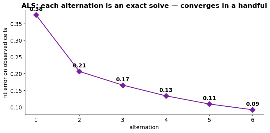
GD needed thousands of tiny steps; ALS reaches the same fit in ~5 exact, parallelisable solves.
Going non-linear: the Autoencoder (your first neural net)
Deep learning in one line: layers of “multiply by a matrix, then bend” — Each is linear (like MF); each activation (ReLU, sigmoid) bends it, so the stack does more than one matrix can.
An autoencoder compresses and rebuilds:
encoder squeezes a rating vector to a small bottleneck,
decoder rebuilds the full vector,
trained on the observed ratings only.
The bottleneck is the embedding (like SVD’s factors, but it can bend). This is AutoRec — strip every and it collapses back to MF.
Source
# Annotated AutoRec: rating vector -> encoder -> bottleneck (embedding) -> decoder -> reconstruction.
# Each arrow is a linear map W·x+b FOLLOWED BY a non-linear activation σ — that σ is what beats plain MF.
fig, ax = plt.subplots(figsize=(13.5, 6.2))
ax.set_xlim(0, 14.5); ax.set_ylim(-1.6, 8.4); ax.axis('off')
layers = [('input $x$\n(rating vector)', 1.3, [0.5, 1.5, 2.5, 3.5, 4.5, 5.5, 6.5, 7.5], '#1976d2'),
          ('hidden\n(encoder)', 4.2, [1.5, 2.5, 3.5, 4.5, 5.5, 6.5], '#7b1fa2'),
          ('bottleneck\n= embedding', 7.2, [2.5, 3.5, 4.5, 5.5], '#d32f2f'),
          ('hidden\n(decoder)', 10.2, [1.5, 2.5, 3.5, 4.5, 5.5, 6.5], '#7b1fa2'),
          ('output $\\hat x$\n(reconstruction)', 13.1, [0.5, 1.5, 2.5, 3.5, 4.5, 5.5, 6.5, 7.5], '#388e3c')]
for idx, (name, x, ys, col) in enumerate(layers):
    r = 0.22 if len(ys) > 5 else 0.28
    for y in ys:
        ax.add_patch(plt.Circle((x, y), r, facecolor=col, edgecolor='white', lw=1.5, zorder=3))
    ax.text(x, -1.15, name, ha='center', fontsize=11, fontweight='bold', color=col)
    if idx < len(layers) - 1:
        _, nx, nys, _ = layers[idx + 1]
        nr = 0.22 if len(nys) > 5 else 0.28
        for y in ys:
            for ny in nys:
                ax.plot([x + r, nx - nr], [y, ny], color='gray', alpha=0.07, lw=0.5)
        ax.annotate('', xy=((x + nx) / 2 + 0.5, 7.7), xytext=((x + nx) / 2 - 0.5, 7.7),
                    arrowprops=dict(arrowstyle='->', color='#333', lw=1.4))
        ax.text((x + nx) / 2, 8.05, r'$\sigma(Wx{+}b)$', ha='center', fontsize=10, color='#333', fontweight='bold')
ax.add_patch(plt.Rectangle((6.5, 1.9), 1.4, 4.2, facecolor='#ffebee',
                           edgecolor='#d32f2f', lw=2, ls='--', alpha=0.45, zorder=1))
ax.text(7.2, 0.55, 'every arrow: multiply by a weight matrix, then bend with a non-linear  $\\sigma$  (ReLU / sigmoid)',
        ha='center', fontsize=11, color='#333', bbox=dict(boxstyle='round', facecolor='#fffde7', edgecolor='#fbc02d'))
ax.set_title('Autoencoder = compress a rating vector to a bottleneck, then reconstruct it', fontweight='bold')
plt.tight_layout()
plt.show()
print('The bottleneck activations are the embedding; the σ on every layer is what lets it out-predict linear MF.')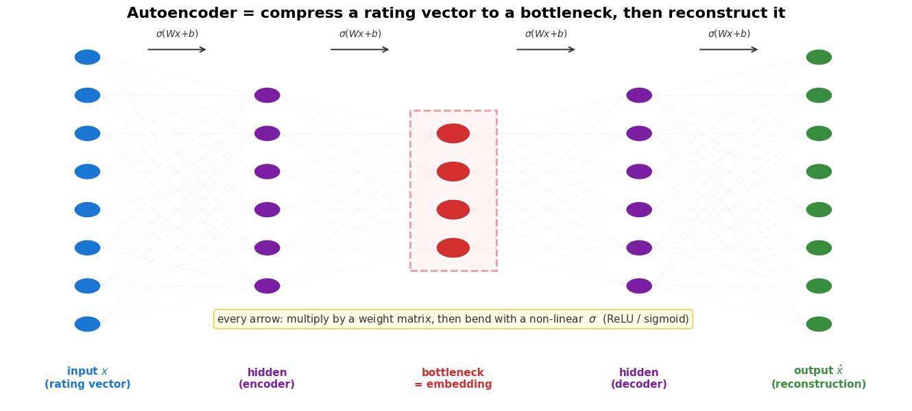
The bottleneck activations are the embedding; the σ on every layer is what lets it out-predict linear MF.
Why “non-linear”? The activation functions
Stack two linear layers and you get — still one linear map, no more powerful than MF. The activation wedged between them is what unlocks new shapes: ReLU , sigmoid, . A single hidden layer of ReLUs can already bend into essentially any curve.
Source
# Left: the activation functions (the 'bend'). Right: why a deep net needs them at all.
xs = np.linspace(-6, 6, 400)
fig, (a1, a2) = plt.subplots(1, 2, figsize=(14, 5))
a1.plot(xs, np.maximum(0, xs), color='#1976d2', lw=2.5, label='ReLU  max(0, x)')
a1.plot(xs, 1 / (1 + np.exp(-xs)), color='#388e3c', lw=2.5, label='sigmoid')
a1.plot(xs, np.tanh(xs), color='#d32f2f', lw=2.5, label='tanh')
a1.axhline(0, color='gray', lw=0.6); a1.axvline(0, color='gray', lw=0.6)
a1.set_title('Activation functions — the "bend"', fontweight='bold')
a1.set_xlabel('x'); a1.legend(); a1.spines[['top', 'right']].set_visible(False)

xt = np.linspace(-3, 3, 300)
target = np.sin(1.3 * xt) + 0.25 * xt                       # a curvy function to fit
centers = np.linspace(-3, 3, 9)
Phi = np.hstack([np.maximum(0, xt[:, None] - centers[None, :]), np.ones((len(xt), 1))])   # ReLU features
w, *_ = np.linalg.lstsq(Phi, target, rcond=None)
nonlin = Phi @ w                                            # 1 ReLU hidden layer -> bends to the curve
lin = np.polyval(np.polyfit(xt, target, 1), xt)            # any stack of linear layers -> just a line
a2.plot(xt, target, color='#333', lw=2.5, label='target (curved)')
a2.plot(xt, lin, color='#1976d2', lw=2.2, ls='--', label='stacked linear layers → still a line')
a2.plot(xt, nonlin, color='#d32f2f', lw=2.2, label='one ReLU hidden layer → bends to fit')
a2.set_title('Why depth needs activations', fontweight='bold')
a2.set_xlabel('x'); a2.legend(loc='upper left', fontsize=10); a2.spines[['top', 'right']].set_visible(False)
plt.tight_layout()
plt.show()
print('No activation → depth buys nothing (W₂W₁ is one matrix). Add σ → the network can model interactions MF cannot.')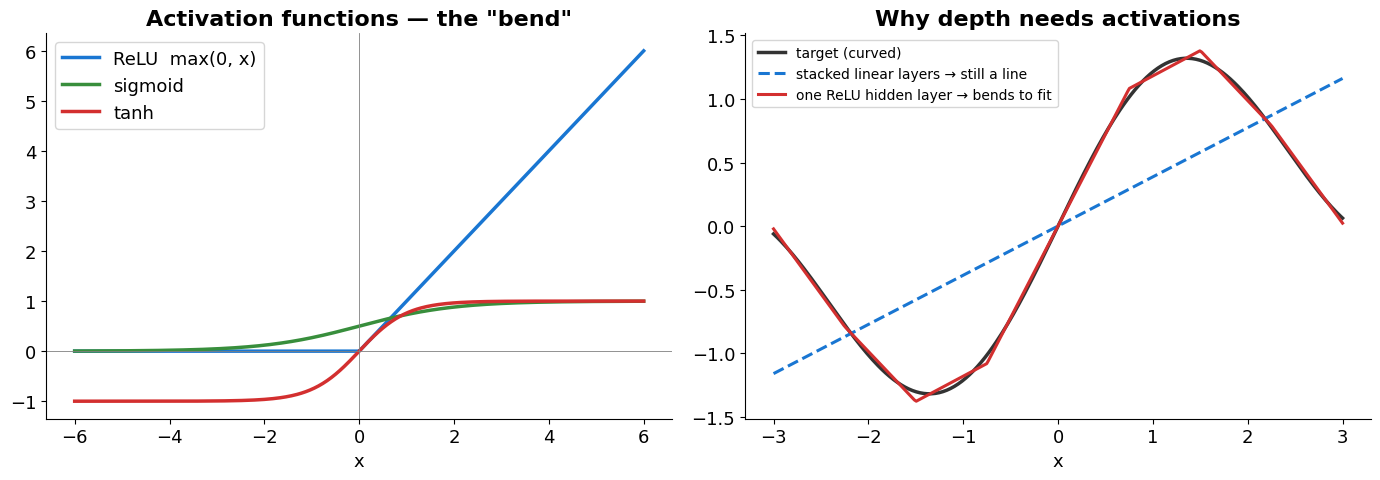
No activation → depth buys nothing (W₂W₁ is one matrix). Add σ → the network can model interactions MF cannot.
The pay-off: autoencoder vs. matrix factorization
Fair test: hide a random 10% of ratings, train both on the rest, predict the hidden ones, score RMSE (lower = better). Two clean code blocks — MF (a library) and the autoencoder (PyTorch) — each with a table of the rating we hid vs what the model guessed.
Source
# (plumbing) Hide a random 10% of ratings as the TEST set; both models train on the remaining 90%.
train_df, test_df = train_test_split(ratings, test_size=0.10, random_state=42)
mu = train_df['rating'].mean()
Rtr = np.zeros((n_users, n_movies), np.float32)                       # 90% train matrix (hidden cells = 0)
Rtr[train_df['user_idx'].values, train_df['movie_idx'].values] = train_df['rating'].values
y_true = test_df['rating'].values                                     # the ratings we hid, for scoring
Model 1 — Matrix Factorization (SVD via the Surprise library, with the from-scratch version beside it)
# Matrix factorization two ways — both learn a k-dim vector for every user & every movie from the 90%.

# (a) the easy way: the Surprise library wraps the whole SVD recipe in a few lines.
#     (it also fits per-user/per-item bias terms and uses k=50, so it scores a little better than the
#      plain k=40, no-bias version in (b) — that gap is the biases, not a different algorithm.)
from surprise import SVD, Dataset, Reader
reader = Reader(rating_scale=(0.5, 5.0))
trainset = Dataset.load_from_df(train_df[['userId', 'movieId', 'rating']], reader).build_full_trainset()
mf = SVD(n_factors=50, n_epochs=30, random_state=42).fit(trainset)
mf_pred = np.array([mf.predict(u, i).est for u, i in zip(test_df['userId'], test_df['movieId'])])

# (b) the same thing from scratch (for information): exactly the SGD we derived, r̂ = μ + p·q.
mu = train_df['rating'].mean()
P = np.random.normal(0, 0.1, (n_users, 40))                     # one 40-dim vector per user
Q = np.random.normal(0, 0.1, (n_movies, 40))                    # one 40-dim vector per movie
for epoch in range(15):
    for u, i, r in zip(train_df['user_idx'], train_df['movie_idx'], train_df['rating']):
        e = r - (mu + P[u] @ Q[i])                              # ① error
        P[u] += 0.01 * (e * Q[i] - 0.05 * P[u])                 # ④ the update rule (user, then item)
        Q[i] += 0.01 * (e * P[u] - 0.05 * Q[i])
np_pred = mu + (P[test_df['user_idx'].values] * Q[test_df['movie_idx'].values]).sum(1)

mf_rmse = np.sqrt(np.mean((mf_pred - y_true) ** 2))             # we use the library version below
np_rmse = np.sqrt(np.mean((np_pred - y_true) ** 2))
print(f'MF test RMSE  —  Surprise library: {mf_rmse:.3f}   |   from-scratch numpy (μ + p·q): {np_rmse:.3f}')
MF test RMSE — Surprise library: 0.883 | from-scratch numpy (μ + p·q): 0.910
Source
# (hidden) A few hidden ratings next to the MF prediction.
def show_predictions(pred, rmse, model_name, color):
    samp = test_df.head(9).merge(movies[['movieId', 'title']], on='movieId', how='left').reset_index(drop=True)
    rows = []
    for k, row in samp.iterrows():
        t = str(row['title']); t = t[:30] + '…' if len(t) > 31 else t
        rows.append([t, f"{row['rating']:.1f}", f'{pred[k]:.2f}'])
    fig, ax = plt.subplots(figsize=(10, 3.6)); ax.axis('off')
    tbl = ax.table(cellText=rows, colLabels=['movie (rating we hid)', 'true', f'{model_name}\npredicts'],
                   cellLoc='center', loc='center', colWidths=[0.62, 0.18, 0.20])
    tbl.auto_set_font_size(False); tbl.set_fontsize(11); tbl.scale(1, 1.7)
    for (r, c), cell in tbl.get_celld().items():
        cell.set_edgecolor('#cccccc')
        if r == 0:
            cell.set_text_props(fontweight='bold', color='white'); cell.set_facecolor(color)
        elif c == 0:
            cell.set_text_props(ha='left'); cell.PAD = 0.03
    ax.set_title(f'{model_name}: predicting the ratings we hid     (test RMSE = {rmse:.3f})',
                 fontweight='bold', fontsize=13)
    plt.tight_layout(); plt.show()

show_predictions(mf_pred, mf_rmse, 'Matrix Factorization', '#1976d2')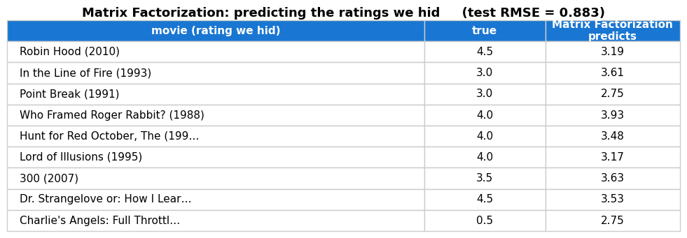
Model 2 — Autoencoder (AutoRec in PyTorch)
# Autoencoder (AutoRec) in PyTorch: feed each movie's rating column, reconstruct it; the bottleneck bends.
import torch
import torch.nn as nn
torch.manual_seed(0)

X = torch.tensor(Rtr.T)                 # one row per MOVIE = its ratings from all users
seen = (X > 0).float()                  # 1 where a rating exists

class AutoRec(nn.Module):
    def __init__(self, n_users, hidden=500):
        super().__init__()
        self.net = nn.Sequential(
            nn.Dropout(0.5),                                  # "denoising": hide half the inputs while training
            nn.Linear(n_users, hidden), nn.Sigmoid(),        # encode  + non-linear activation σ
            nn.Linear(hidden, n_users))                      # decode back to a full rating column
    def forward(self, x):
        return self.net(x)

ae = AutoRec(n_users)
opt = torch.optim.Adam(ae.parameters(), lr=3e-3, weight_decay=1e-4)
for epoch in range(350):
    loss = (((ae(X) - X) ** 2) * seen).sum() / seen.sum()    # error on observed cells only
    opt.zero_grad(); loss.backward(); opt.step()

ae.eval()
with torch.no_grad():
    recon = ae(X).numpy().T                                  # reconstructed full matrix (users x movies)
ae_pred = recon[test_df['user_idx'].values, test_df['movie_idx'].values]
ae_rmse = np.sqrt(np.mean((ae_pred - y_true) ** 2))
print(f'Autoencoder — test RMSE on the hidden ratings: {ae_rmse:.3f}')
Autoencoder — test RMSE on the hidden ratings: 0.835
Source
# (hidden) Same hidden ratings, now the autoencoder's guesses.
show_predictions(ae_pred, ae_rmse, 'Autoencoder', '#388e3c')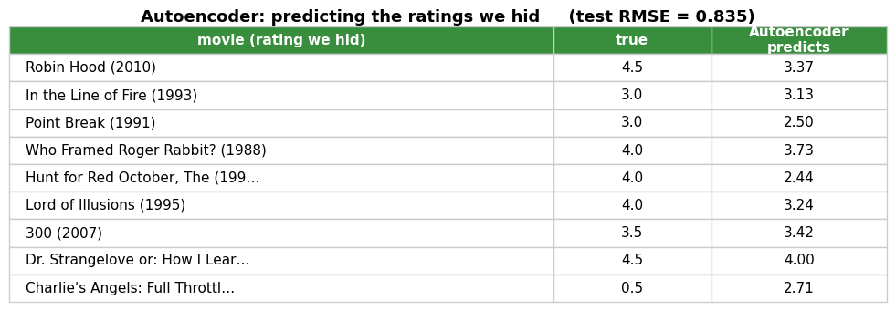
Source
# (hidden) The verdict: test RMSE on the identical hidden 10%.
rmse_base = float(np.sqrt(np.mean((mu - y_true) ** 2)))
fig, ax = plt.subplots(figsize=(9, 5))
names = ['Global-mean\nbaseline', 'Matrix\nFactorization', 'Autoencoder\n(AutoRec)']
vals = [rmse_base, float(mf_rmse), float(ae_rmse)]
bars = ax.bar(names, vals, color=['#90a4ae', '#1976d2', '#388e3c'], edgecolor='white', width=0.6)
for b, v in zip(bars, vals):
    ax.text(b.get_x() + b.get_width() / 2, v + 0.008, f'{v:.3f}', ha='center', fontsize=15, fontweight='bold')
ax.set_ylim(0.7, max(vals) + 0.08)
ax.set_ylabel('test RMSE on the hidden 10%  (lower = better)')
ax.set_title('Same data, same 10% hidden: the non-linear autoencoder predicts best', fontweight='bold')
ax.spines[['top', 'right']].set_visible(False)
plt.tight_layout()
plt.show()
print(f'baseline {rmse_base:.3f}  →  MF {mf_rmse:.3f}  →  AutoRec {ae_rmse:.3f}   '
      f'(AutoRec beats MF by {100 * (mf_rmse - ae_rmse) / mf_rmse:.0f}%).  '
      f'Illustrative, not a capacity-matched benchmark — the AE has more parameters (500 hidden + dropout).')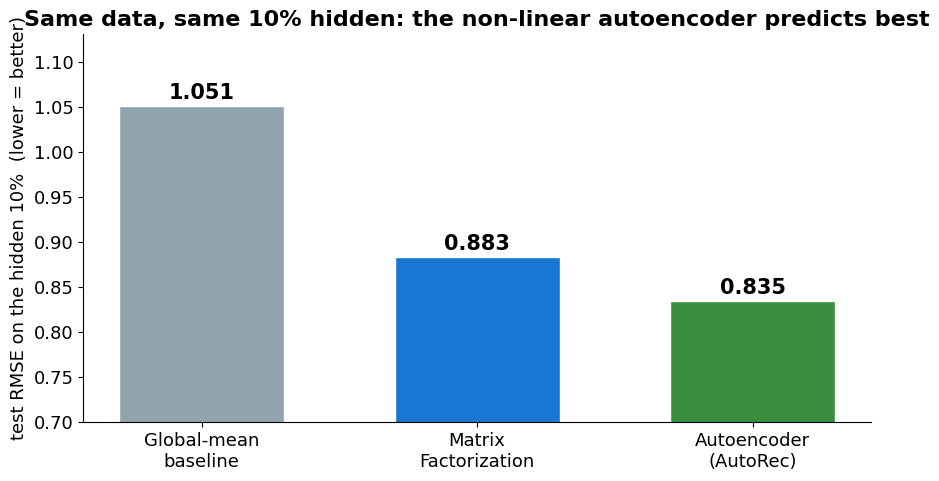
baseline 1.051 → MF 0.883 → AutoRec 0.835 (AutoRec beats MF by 5%). Illustrative, not a capacity-matched benchmark — the AE has more parameters (500 hidden + dropout).
The bridge to Session 9 — the cold-start wall
Transductive = the model only knows the IDs it trained on.
Inductive = a function that makes a vector for any input, even an unseen one.
MF is fully transductive: a user/movie is a learned row — a brand-new ID has no row, so you must retrain.
AutoRec goes half a step further: it eats a rating vector. We feed it each movie’s ratings (so the input width is the user list), and a new movie that already has a few ratings gets predictions in one forward pass — no retraining. But a brand-new user, or a movie with zero ratings, still cold-starts.
The real fix builds the vector from content (title, plot, poster) — so even a movie with zero ratings gets an embedding. That inductive leap is Session 9 (Sentence Transformers): data → vectors → latent space → retrieval.
Key Takeaways
Two roads: predict a cell (Bayes — a number) vs. learn vectors (embeddings).
Matrix factorization — users & items in one shared space.
SVD is the optimal linear factorization, but needs a full matrix; filling holes with 0 is biased.
Gradient Descent & ALS fit on observed ratings only (+ regularization) — same goal, two optimizers.
The rows of are embeddings — cosine similarity (Session 7) now applies to learned vectors.
Autoencoders are the non-linear upgrade — the activation lets them beat MF on held-out ratings.
Transductive → cold start. Next: inductive neural embeddings (Session 9).
→ Now switch to the practice notebook: SVD & SGD from scratch, then build an AutoRec.