Session 3: Data Quality
Learning goals
Data Quality Dimensions
Data Quality Checks
Data Profiling
Missing Values
Realistic Missingness Patterns
Imputation
Outlier detection
Redaction
Why Data Quality
Poor data quality costs the US economy ~$3.1 trillion/year (IBM, 2016)
Causes: Wasted time, Operational inefficiencies, Trust issues
ML models inherit and amplify data defects Sculley et al. (2015)
Legal Perspective (personal rights / privacy)
Data Quality Standards
ISO 8000 mandate International Organization for Standardization (ISO) (2022)
Artificial intelligence — Data quality for analytics and machine learning (ML) International Organization for Standardization (2023)
Systems and software engineering – Systems and software Quality Requirements and Evaluation (SQuaRE) – Measurement of data quality International Organization for Standardization (2015)
Data Quality is difficult to automate (Biessmann et al. (2021) and Schelter et al. (2018))
GDPR and HIPAA
| Aspect | GDPR (General Data Protection Regulation) | HIPAA (Health Insurance Portability and Accountability Act) |
|---|---|---|
| Scope | Protects personal data of EU citizens, globally | Protects health information of US patients |
| Data Covered | Any personal data (name, email, IP, etc.) | Protected Health Information (PHI) only |
| Who Must Comply | Any organization processing EU residents’ data | US healthcare providers, insurers, and business associates |
| Key Rights | Right to access, correct, delete, and port data | Right to access, amend, and restrict PHI disclosure |
| Penalties | Up to 4% of global revenue or €20M, whichever is higher | Up to $1.5M per violation, per year |
| Breach Notification | Within 72 hours of discovery | Within 60 days of discovery |
ISO Data Quality Standards
ISO/IEC 25024:2015 – Data Quality Measurement International Organization for Standardization (2015)
Framework to quantitatively measure various aspects of data quality
Accuracy, completeness, consistency, and timeliness
ISO 8000 Series – Data Quality Management and Exchange International Organization for Standardization (ISO) (2022)
Requirements for managing and exchanging master data to improve data quality across organizations.
Emphasizes the importance of data quality in enhancing business processes and decision-making.
ISO/IEC 5259 Series – Data Quality for Analytics and Machine Learning (ML) International Organization for Standardization (2023)
Focuses on ensuring data quality for AI and ML applications
Provides frameworks and measurable characteristics to help organizations effectively manage their data quality in analytical workflows
ISO/IEC 25024:2015 – Data Quality Measurement
Example: Consider a company that collects customer data for its marketing campaigns. Using ISO/IEC 25024:2015, the company can measure:
Accuracy: By comparing customer addresses in their database against a reliable external database (e.g., postal service data), they can determine the percentage of addresses that are valid.
Completeness: The company can calculate the percentage of customer records that have complete information, such as name, address, email, and phone number. If they find that only 70% of records have a valid phone number, they can work on strategies to gather this missing data.
Timeliness: The company may assess how current their data is by checking the age of records. If most records are over two years old, they may need to implement a regular update process to ensure data remains relevant.
ISO 8000 Series – Data Quality Management and Exchange
Example: A manufacturing company that manages a complex supply chain can apply the ISO 8000 standards to improve the quality of their product master data:
Data Provenance: The company can implement tracking for each product’s origin, including details about the supplier, production date, and batch number. This ensures that all stakeholders have access to accurate historical data, which is critical for quality control and compliance.
Interoperability: When exchanging data with suppliers and customers, the company can adopt standardized formats as per ISO 8000. For instance, using a standardized product identifier (like GTIN) allows seamless integration of data between their systems and those of suppliers, reducing errors in product information.
Accuracy and Consistency: They can regularly audit their product data against sales records and inventory systems, ensuring that product descriptions, specifications, and prices are consistent across all platforms. If discrepancies are found, they can initiate corrective actions to maintain high data quality standards.
ISO/IEC 5259 Series – Data Quality for Analytics and ML
Example: A financial institution uses machine learning algorithms to detect fraudulent transactions. Applying the ISO/IEC 5259 standards, the institution can:
Establish a Data Quality Model: Define what constitutes high-quality transaction data (e.g., accuracy, consistency, and relevance) and create a scorecard to evaluate the quality of incoming transaction data.
Assess Completeness: Before inputting data into their ML model, they can check for missing fields, such as the merchant category code (MCC), which could be crucial for identifying fraud patterns. If many transactions lack this information, they may need to implement a validation step to ensure all necessary fields are populated.
Monitor Data Consistency: They can regularly review data from different sources for discrepancies. If one data source lists a transaction amount as 100 Eur while another source lists it as 90 Eur, the institution can flag this for review, ensuring that only consistent data is used in their fraud detection models.
6 Data Quality Dimensions Wang & Strong (1996)
| Dimension | Question |
|---|---|
| Completeness | Are all values present? |
| Uniqueness | Are records deduplicated? |
| Consistency | Do values obey rules/formats? |
| Accuracy | Do values reflect reality? |
| Timeliness | Is data current enough? |
| Validity | Do values match expected domains? |
Wang & Strong (1996)
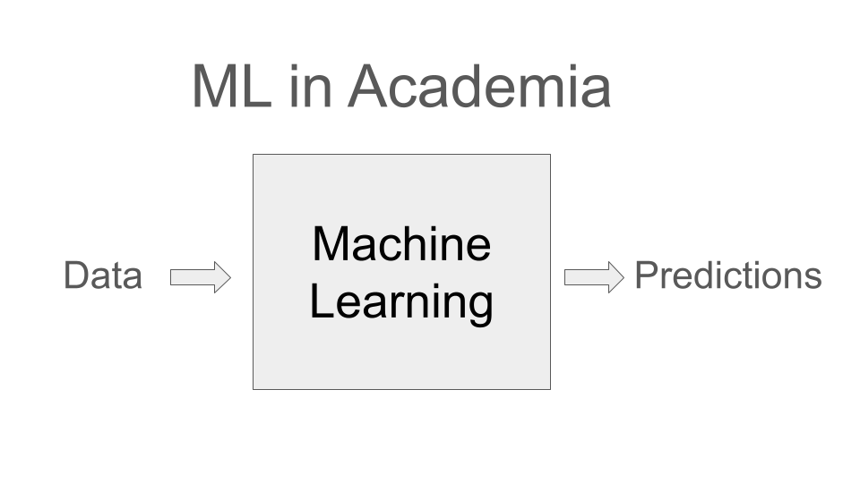
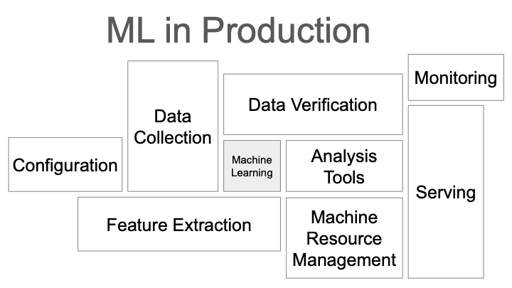
adapted from Sculley et al. (2015)
Data Quality Monitoring
Let’s consider a simple dataset of employee information and insert some outliers:
import pandas as pd
import numpy as np

np.random.seed(42)
n = 200

df = pd.DataFrame({
    'employee_id': list(range(1, n + 1)) + [5, 12],          # duplicates
    'name':        ['Alice', 'Bob'] * (n // 2) + [None, 'Bob'],
    'age':         np.random.randint(22, 65, n + 2).tolist(),
    'salary':      np.random.normal(55000, 12000, n + 2).tolist(),
    'department':  np.random.choice(['HR', 'Eng', 'Sales', None], n + 2).tolist(),
    'hire_date':   pd.date_range('2015-01-01', periods=n + 2, freq='W'),
})

# Inject outliers
df.loc[10, 'salary'] = 999_999
df.loc[20, 'age']    = -5

print(f'Shape: {df.shape}')
df.head(3)
Shape: (202, 6)
Automated Profiling with ydata-profiling
Formerly known as
pandas-profiling— generates a comprehensive HTML report covering all quality dimensions in one call.
import sys
import importlib.util

# This manually satisfies the 'import pkg_resources' requirement in memory
if importlib.util.find_spec("pkg_resources") is None:
    try:
        import setuptools.extern
        from setuptools import pkg_resources
        sys.modules["pkg_resources"] = pkg_resources
        print("Polyfill: pkg_resources successfully mapped from setuptools.")
    except ImportError:
        # Emergency fallback to pip's internal copy
        import pip._vendor.pkg_resources as pkg_resources
        sys.modules["pkg_resources"] = pkg_resources
        print("Polyfill: pkg_resources successfully mapped from pip vendor.")

# NOW this will work
from ydata_profiling import ProfileReport
from ydata_profiling import ProfileReport
profile = ProfileReport(
df,
title='Employee Dataset Quality Report',
explorative=True,
minimal=False,
)
# Save to HTML for sharing
profile.to_file('data_quality_report.html')
# Render inline in the notebook
profile.to_notebook_iframe()100%|██████████| 6/6 [00:00<00:00, 878.02it/s]
Data Quality Dimensions
completeness = 1 - df.isnull().mean()

print('=== Completeness per column ===')
print(completeness.round(3).to_string())

print(f'\nOverall completeness: {completeness.mean():.2%}')
=== Completeness per column ===
employee_id 1.000
name 0.995
age 1.000
salary 1.000
department 0.767
hire_date 1.000
Overall completeness: 96.04%
# Visualise missing pattern
import matplotlib.pyplot as plt
missing = df.isnull().sum()
missing[missing > 0].plot(kind='bar', color='#e74c3c', title='Missing value counts')
plt.tight_layout()
plt.show()n_dupes = df.duplicated(subset='employee_id').sum()
uniqueness = 1 - n_dupes / len(df)
print(f'Duplicate employee_id rows : {n_dupes}')
print(f'Uniqueness score : {uniqueness:.2%}')
# Inspect
df[df.duplicated(subset='employee_id', keep=False)].sort_values('employee_id')Duplicate employee_id rows : 2
Uniqueness score : 99.01%
Validity & Consistency
Values must conform to domain rules and referential constraints.
Examples:
agemust be in[18, 80]salarymust be> 0departmentmust be in a known set
rules = {
    'age_valid':        df['age'].between(18, 80),
    'salary_positive':  df['salary'] > 0,
    'dept_known':       df['department'].isin(['HR', 'Eng', 'Sales']),
}

for rule_name, mask in rules.items():
    pass_rate = mask.mean()
    fail_count = (~mask).sum()
    print(f'{rule_name:<20} pass={pass_rate:.2%}  violations={fail_count}')
age_valid pass=99.50% violations=1
salary_positive pass=100.00% violations=0
dept_known pass=76.73% violations=47
Aggregated Quality Score
Sometimes it can be helpful to aggregate data quality metrics
Pipino et al. (2002) propose a composite score:
where is the weight for dimension and is its metric value.
scores = {
    'Completeness': completeness.mean(),
    'Uniqueness':   uniqueness,
    'Validity_age': df['age'].between(18, 80).mean(),
    'Validity_sal': (df['salary'] > 0).mean(),
    'Validity_dept': df['department'].isin(['HR','Eng','Sales']).mean(),
}

weights = [0.25, 0.25, 0.15, 0.15, 0.20]  # domain-defined
composite = sum(w * v for w, v in zip(weights, scores.values()))

print('--- Dimension Scores ---')
for k, v in scores.items():
    print(f'  {k:<20} {v:.2%}')
print(f'\n  Composite DQ Score   {composite:.2%}')
--- Dimension Scores ---
Completeness 96.04%
Uniqueness 99.01%
Validity_age 99.50%
Validity_sal 100.00%
Validity_dept 76.73%
Composite DQ Score 94.03%
Accuracy / Outlier Detection
The accuracy dimension of data quality refers to statistical properties of data
Simple outlier detection: parametric tests (z-scoring)
Statisticians / ML researchers develop anomaly / outlier detection methods
Declarative Data Quality Test
Similiar to how unit tests work for software, we can define data quality tests to automatically check for issues in our datasets.
Testing all data quality dimensions is difficult
Some are easy to test
Libraries provide declarative language to define tests
Defining tests remains manual work
deequ
val verificationResult = VerificationSuite()
    .onData(data)
    .addCheck(
        Check(CheckLevel.Error, "unit testing my data")
            .hasSize(_ == 5) // we expect 5 rows
            .isComplete("id") // should never be NULL
            .isUnique("id") // should not contain duplicates
            .isComplete("name") // should never be NULL
            // should only contain the values "high" and "low"
            .isContainedIn("priority", Array("high", "low"))
            // at least half of the descriptions should contain a url
            .containsURL("description", _ >= 0.5)
            // half of the items should have less than 10 views
            .hasApproxQuantile("numViews", 0.5, _ <= 10))
    .run()```

@schelter2018automating
deequ Workflow:
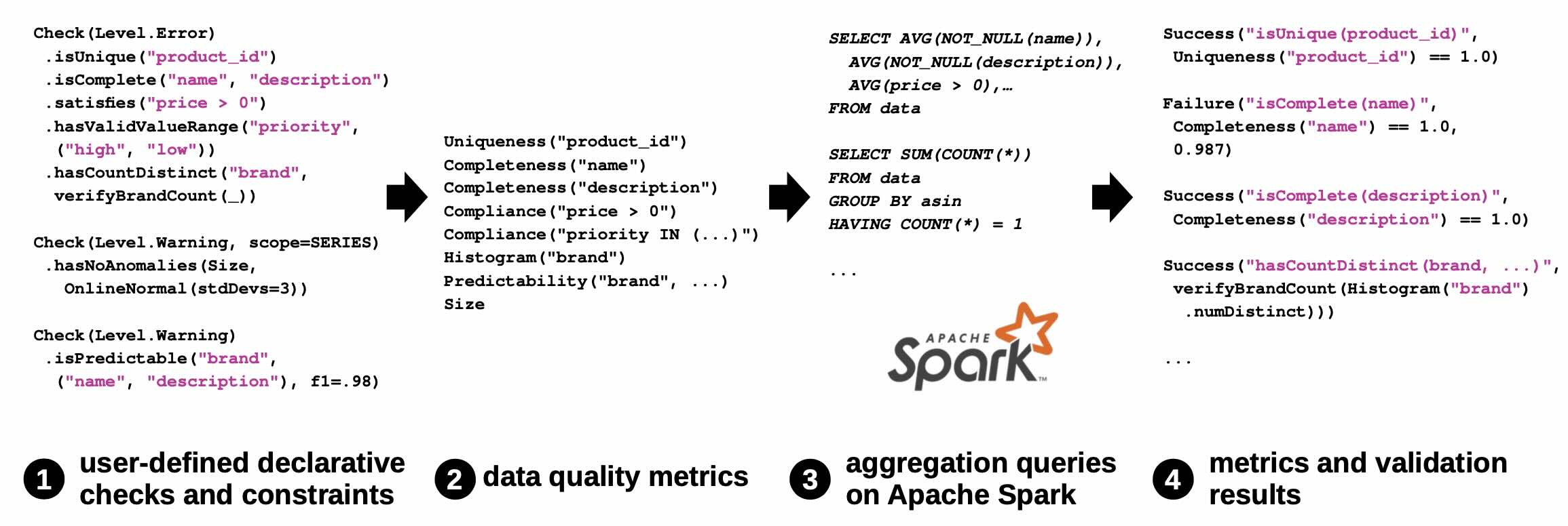
great_expectations
Similar to deequ (Schelter et al) for Scala/Spark, the python library Great Expectations allows you to define, document, and validate data contracts declaratively.
Conceptually:
EXPECT column X TO HAVE values between A and B
EXPECT column Y TO NOT BE NULL
EXPECT table TO HAVE exactly N columns
Schelter et al. (2018)
import great_expectations as gx

context = gx.get_context()

# 1. Access via data_sources
ds = context.data_sources.add_pandas('my_ds')
da = ds.add_dataframe_asset('employee_data')

# 2. FIX: In 1.x, use 'options' to pass the dataframe
batch = da.build_batch_request(options={'dataframe': df})

# 3. FIX: Use the 1.x suite manager
suite = context.suites.add(gx.ExpectationSuite(name='employee_suite'))

# 4. Use the batch_request as before
validator = context.get_validator(batch_request=batch, expectation_suite=suite)

# Define expectations
validator.expect_column_values_to_not_be_null('employee_id')
validator.expect_column_values_to_be_between('age', min_value=18, max_value=80)
validator.expect_column_values_to_be_in_set('department', ['HR', 'Eng', 'Sales'])
validator.expect_column_values_to_be_unique('employee_id')

results = validator.validate()
print(f'Success: {results.success}')
print(f'Passed: {results.statistics["successful_expectations"]} / '
f'{results.statistics["evaluated_expectations"]}')Success: False
Passed: 2 / 4
Anomaly Detection
Anomaly detection is an important task
Anomaly detection is difficult:
We usually don’t know what is normal/anomalous
If we have examples of anomalies, they are usually very rare
For evaluation, we can use classification metrics but we need labels for that
There are great libraries for anomaly detection:
Simple Anomaly Detection
Statistical outliers can indicate data entry errors or sensor faults.
Z-score method Iglewicz & Hoaglin (1993) :
IQR method (more robust to non-normal distributions):
from scipy import stats

for col in ['salary', 'age']:
    z = np.abs(stats.zscore(df[col].dropna()))
    out_idx = df[col].dropna().index[z > 3]
    print(f'[Z-score] {col} outliers ({len(out_idx)}):')
    print(df.loc[out_idx, ['employee_id', col]], '\n')

    Q1, Q3 = df[col].quantile([0.25, 0.75])
    IQR = Q3 - Q1
    iqr_mask = (df[col] < Q1 - 1.5*IQR) | (df[col] > Q3 + 1.5*IQR)
    print(f'[IQR]     {col} outliers: {iqr_mask.sum()}\n')
[Z-score] salary outliers (1):
employee_id salary
10 11 999999.0
[IQR] salary outliers: 1
[Z-score] age outliers (1):
employee_id age
20 21 -5
[IQR] age outliers: 1
Another view: Parametric Distributions
Consider univariate data drawn from a normal distribution .
import matplotlib
matplotlib.get_backend()'module://matplotlib_inline.backend_inline'mu = 2
sigma = 3
x = np.random.randn(1000) * sigma + mu
plt.hist(x);What’s an anomalous data point?
The likelihood of each sample under this distribution is given by
So you can compute the likelihood of any given data point as:
def gauss_likelihood(x, mu, sigma):
    '''
    Computes the likelihood of x assuming x is from a
    normal distribution with mean mu and standard deviation sigma
    '''
    denom = (np.sqrt(2.*np.pi)*sigma)
    num = np.exp(-.5*((x - mu) / sigma)**2)
    return num/denom

print(gauss_likelihood(2., mu,sigma))

# alternatively you can use the scipy.stats package
from scipy.stats import norm
my_gauss = norm(mu, sigma)
print(my_gauss.pdf(2))
0.1329807601338109
0.1329807601338109
Defining Anomaly
Given a data point and a (not necessarily generative) model of your data, you can define a threshold for what’s an anomaly.
For instance, a common threshold is to assume that data points for which or are anomalous.
steps = np.arange(-10,100)
plt.plot(x, gauss_likelihood(x,mu,sigma),'.');
plt.plot([-7.5,12.5],[.05,.05],'r--')
plt.plot([-7.5,12.5],[.01,.01],'k--')
plt.legend(['p(x)','0.05','0.01'])
Multivariate Anomaly Detection
Simple Parametric Approach: Assuming Gaussian Data
Sophisticated Non-parametric: Isolation Forest
Example taken from Alexandre Gramforts sklearn tutorial
from sklearn.datasets import make_moons, make_blobs
from sklearn.covariance import EllipticEnvelope
from sklearn.ensemble import IsolationForest

plt.rcParams['contour.negative_linestyle'] = 'solid'
plt.rcParams['figure.figsize'] = [5, 5]

n_samples = 300
outliers_fraction = 0.15
n_outliers = int(outliers_fraction * n_samples)
n_inliers = n_samples - n_outliers

anomaly_algorithms = [
    ("Robust covariance", EllipticEnvelope(contamination=outliers_fraction)),
    ("Isolation Forest", IsolationForest(contamination=outliers_fraction,
                                         random_state=42))]

# Define datasets
blobs_params = dict(random_state=0, n_samples=n_inliers, n_features=2)
datasets = [
    make_blobs(centers=[[0, 0], [0, 0]], cluster_std=0.5,
               **blobs_params)[0],
    make_blobs(centers=[[2, 2], [-2, -2]], cluster_std=[0.5, 0.5],
               **blobs_params)[0],
    4. * (make_moons(n_samples=n_samples, noise=.05, random_state=0)[0] -
          np.array([0.5, 0.25]))]

# Compare given classifiers under given settings
xx, yy = np.meshgrid(np.linspace(-7, 7, 150),
                     np.linspace(-7, 7, 150))

plot_num = 1
rng = np.random.RandomState(42)
for i_dataset, X in enumerate(datasets):
    # Add outliers
    X = np.concatenate([X, rng.uniform(low=-6, high=6,
                       size=(n_outliers, 2))], axis=0)

    for name, algorithm in anomaly_algorithms:

        plt.subplot(len(datasets), len(anomaly_algorithms), plot_num)
        if i_dataset == 0:
            plt.title(name, size=12)

        y_pred = algorithm.fit(X).predict(X)

        # plot the levels lines and the points
        Z = algorithm.predict(np.c_[xx.ravel(), yy.ravel()])
        Z = Z.reshape(xx.shape)
        plt.contour(xx, yy, Z, levels=[0], linewidths=2, colors='black')

        colors = np.array(['#377eb8', '#ff7f00'])
        plt.scatter(X[:, 0], X[:, 1], s=10, color=colors[(y_pred + 1) // 2])

        plt.xlim(-7, 7)
        plt.ylim(-7, 7)
        plt.xticks(())
        plt.yticks(())
        plot_num += 1

plt.show()
Missing Values
There are three main options how to deal with missing values:
drop rows with missing values
probably ok, if you have enough data
but can introduce biases in your data that bias your downstream models
replace missing values with placeholder symbol
probably ok, if you have a nonlinear downstream model and the right type of missingness (MAR or MNAR)
but sometimes you are really interested in the missing values
impute missing values with some ML model
import pandas as pd
import numpy as np

berlin_population_dict = {
 '1945': 2807405,
 '1950': 3336026,
 '1955': None,
 '1960': 3274016,
 '1965': np.nan, # pandas understands different missing values
 '1970': 3208719}

population_w_nans = pd.Series(berlin_population_dict)
population_w_nans
1945 2807405.0
1950 3336026.0
1955 NaN
1960 3274016.0
1965 NaN
1970 3208719.0
dtype: float64Dropping rows
Easy with boolean indexing in pandas or numpy
# Check for missing values
population_w_nans.isnull()
1945 False
1950 False
1955 True
1960 False
1965 True
1970 False
dtype: bool# Filter out missing values using boolean indexing
population_w_nans[~population_w_nans.isnull()]1945 2807405.0
1950 3336026.0
1960 3274016.0
1970 3208719.0
dtype: float64# Filter out missing values using dropna
population_w_nans.dropna()1945 2807405.0
1950 3336026.0
1960 3274016.0
1970 3208719.0
dtype: float64Filling with Placeholder
# Fill missing values with forward fill method
population_w_nans.fillna(method='ffill')
1945 2807405.0
1950 3336026.0
1955 3336026.0
1960 3274016.0
1965 3274016.0
1970 3208719.0
dtype: float64# Fill missing values with median
population_w_nans.fillna(value=population_w_nans.median())1945 2807405.0
1950 3336026.0
1955 3241367.5
1960 3274016.0
1965 3241367.5
1970 3208719.0
dtype: float64Filling with Placeholder in sklearn
This way you’ll be able to replace missing values in ML Pipelines
from sklearn.impute import SimpleImputer
import numpy as np
imp = SimpleImputer(missing_values=np.nan, strategy="most_frequent")
imp.fit_transform(population_w_nans.to_numpy().reshape(-1,1))
array([[2807405.],
[3336026.],
[2807405.],
[3274016.],
[2807405.],
[3208719.]])Imputation
You can also use more sophisticated imputation methods
# some toy data with non-linear dependency between columns
n = 10
x = np.random.randn(n,1)
y = x**2

df = pd.DataFrame(np.hstack([x,y]),columns=['x','f(x)'])

mask = np.random.random((n,1)) > .9
dffrom sklearn.experimental import enable_iterative_imputer
from sklearn.impute import IterativeImputer
import matplotlib.pylab as plt
imp = IterativeImputer(max_iter=10, random_state=0)
X_train = df.loc[mask==0,:].values
imp.fit(X_train)
X_test = df.loc[mask>0,:].values
X_test_imputed = imp.transform(X_test)
plt.figure(figsize=[4,4])
plt.plot(X_train[:,0], X_train[:,1], 'r.',
X_test_imputed[:,0], X_test_imputed[:,1],'b.')
plt.ylabel("f(x)")
plt.xlabel("x");This also works for Tabular Data
| Product | Description | Color |
|---|---|---|
| Shoe | Ideal for running | Black |
| Dress | This yellow dress ... | ? |
| ... | ... | ... |
Biessmann et al. (2019)
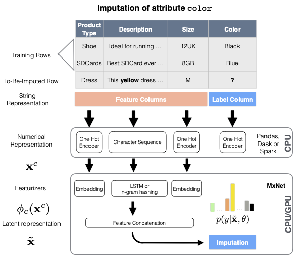
Biessmann et al. (2018)
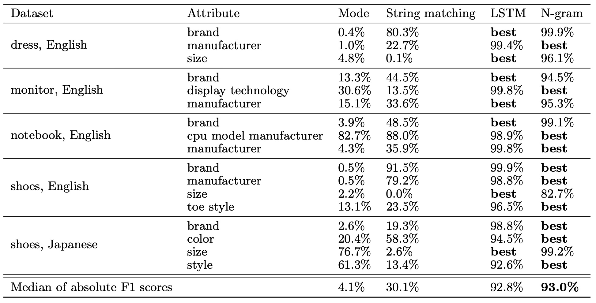
Biessmann et al. (2018)
Realistic Missingness Patterns
Missing Completely at Random (MCAR):
Definition: Missingness is entirely random and unrelated to both observed and unobserved data.
Example: Sensor noise
Missing at Random (MAR):
Definition: Missingness is related to observed data but not to the missing data itself.
Example: Older patients not reporting pain levels, but their pain levels are unrelated to whether they reported.
Missing Not at Random (MNAR):
Definition: Missingness is related to the unobserved data itself.
Example: Higher-income individuals not reporting their income.
Realistic Missingness Patterns as generic error models
We can use these ideas not only for missingness, but for all kinds of errors
Modelling realistic errors in tables Jung et al. (2025)
Detecting realistic error patterns in tables Jung et al. (2025)
Testing ML systems with realistic error patterns
Jäger et al. (2021) and Jäger & Biessmann (2024)
Schelter et al. (2021)
Rukat et al. (2020)
Schelter et al. (2020)
Why should we model Realistic Errors?
Errors are important:
Evaluation of cleaning methods / robustness
Regularization (adding noise to reduce overfitting)
Augmentation (training contrastive learning models, Computer Vision)
Privacy (adding noise to hide sensitive data)
Most error models are oversimplified
Better error models can
Improve training (regularization, augmentation, privacy)
Improve evaluation (more realistic evaluations of robustness)
Yield insights in error generation / provenance
Realistic errors with tab-err
Reference implementation of realistic error mechanisms Towards Realistic Error Models for Tabular Data Jung et al. (2025).
Perturbation of Pandas DataFrames using MCAR/MNAR/MAR for various error types
GitHub: here.
Install tab-err with the command: pip install tab-err
from tab_err import error_mechanism, error_type
import pandas as pd
from sklearn.datasets import load_iris
Load the data
# Load the local iris dataset and name to match UCI ML repo.
iris = load_iris()
df = pd.DataFrame(data=iris.data, columns=[
    'sepal_length', 'sepal_width', 'petal_length', 'petal_width'
])
df['class'] = iris.target_names[iris.target]

df.head()Helper function to display the results
def show_result(original_df: pd.DataFrame, perturbed_df: pd.DataFrame, error_mask: pd.DataFrame | None = None, keys=["original", "perturbed", "error_mask"]) -> pd.DataFrame:
    """Simple helper function to show DataFrames after perturbing them."""
    return (
        pd.concat([original_df, perturbed_df], keys=keys[:2], axis=1)
        if error_mask is None
        else pd.concat([original_df, perturbed_df, error_mask], keys=keys, axis=1)
)APIs
Tab-err includes three APIs depending on the level of control desired.
Low-level API: This API allows for perturbations in one column with a given configuration.
Mid-level API: This API allows for perturbations in multiple columns with a given configuration.
High-level API: This API allows for perturbations in multiple columns and needs only an error rate and the data.
All APIs return a dataframe with the perturbed data and a dataframe with a binary error mask.
Low-Level API
Detailed control
Select the column to perturb
Error mechanism (ECAR, ENAR, EAR)
Error rate
Error type.
In this example, we utilize missing values with the ECAR error type and a 50% error rate on the sepal_width column.
from tab_err.api import low_level

perturbed_data, error_mask = low_level.create_errors(
    df,
    column="sepal_width",
    error_mechanism=error_mechanism.ECAR(),
    error_type=error_type.MissingValue(),
    error_rate=0.5
)
show_result(df, perturbed_data, error_mask).head()Mid-Level API
MidLevelConfig allows detailed but scalable control
In our scenario, we will apply two error models to the sepal_width column and one error model to the class column. In the error applied to the class column, we will use the EAR error mechanism and condition on the petal_width column.
Configuration Specification
from tab_err import ErrorModel
from tab_err.api import MidLevelConfig

config = MidLevelConfig(
        {
            "sepal_width": [
                ErrorModel(
                    error_mechanism=error_mechanism.ECAR(),
                    error_type=error_type.MissingValue(),
                    error_rate=0.5
                    ),
                ErrorModel(
                    error_mechanism=error_mechanism.ENAR(),
                    error_type=error_type.AddDelta({"add_delta_value": 0.1}),
                    error_rate=0.25
                )
                ],
            "class": [
                ErrorModel(
                    error_mechanism=error_mechanism.EAR(
                        condition_to_column="petal_width"
                    ),
                    error_type=error_type.Typo(),
                    error_rate=0.5
                )
            ]
        }
    )
Application of Mid-Level API
from tab_err.api import mid_level

perturbed_data, error_mask = mid_level.create_errors(data=df, config=config)
show_result(df, perturbed_data, error_mask).head()High-Level API
Least user interaction required
Expects data and an error rate.
Applies one error model to each column with a random (but valid) error type and error mechanism.
We will perturb the entire dataframe with a rate of 50%.
from tab_err.api import high_level

perturbed_data, error_mask = high_level.create_errors(data=df, error_rate=0.5)
show_result(df, perturbed_data, error_mask).head()Perturbing and Imputing
# Drop the class column to ensure numeric errors
df = df.drop(columns=["class"])

perturbed_data, error_mask = high_level.create_errors(
        df,
        error_rate=0.20,
        error_mechanisms_to_include=[error_mechanism.ECAR()],
        error_types_to_include=[error_type.MissingValue()]
    )
show_result(df, perturbed_data, error_mask).head()Imputing data
from sklearn.impute import SimpleImputer

imp = SimpleImputer(strategy="mean").set_output(transform="pandas")

df_imputed = imp.fit_transform(perturbed_data)
show_result(df, perturbed_data, df_imputed, keys=["original", "perturbed", "imputed"]).head()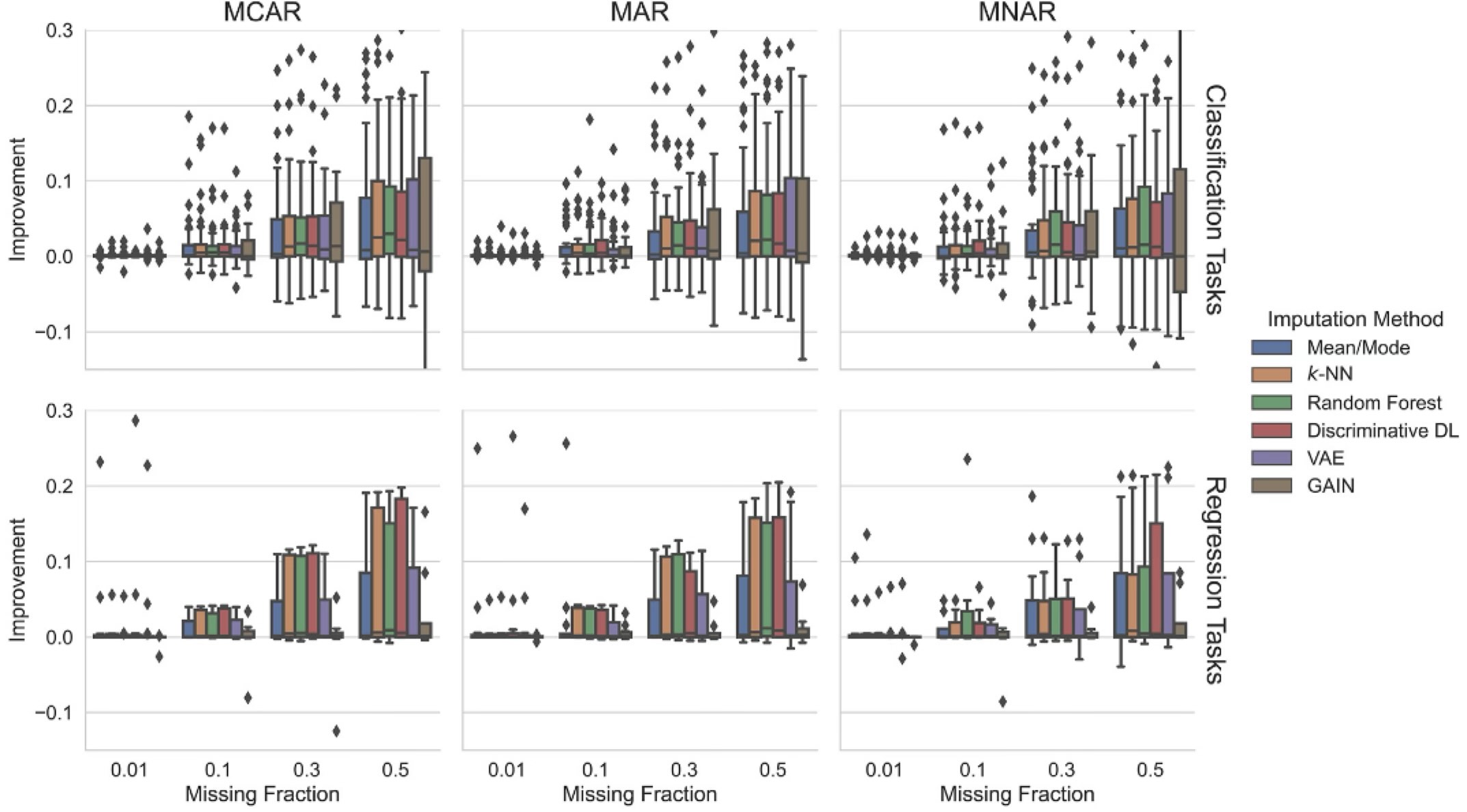
Privacy and redaction
LLMs are popular
Privacy concerns with personally identifying information
Named-Entity Recognition models can redact sensitive information
redaktodemo Saha & Biessmann (2025)
Summary
Data Quality is important
For researchers
For society
For businesses
Data quality monitoring tools help with testing
Automating DQ checks remains challenging
Anna Karenina Principle of Data Quality (due to Charles Sutton):
All healthy data is healthy in the same way. But each broken data set is broken in its own way
- Sculley, D., Holt, G., Golovin, D., Davydov, E., Phillips, T., Ebner, D., Chaudhary, V., Young, M., Crespo, J. F., & Dennison, D. (2015). Hidden technical debt in machine learning systems. Adv. Neural Inf. Process. Syst., 2015-Janua, 2503–2511. http://papers.nips.cc/paper/5656-hidden-technical-debt-in-machine-learning-systems
- Regulation (EU) 2016/679 of the European Parliament and of the Council, (2016). https://eur-lex.europa.eu/legal-content/EN/TXT/?uri=CELEX%253A32016R0679
- Health Insurance Portability and Accountability Act of 1996, (1996). https://www.hhs.gov/hipaa/for-professionals/privacy/laws-regulations/index.html
- International Organization for Standardization (ISO). (2022). Data quality — Part 1: Overview. ISO. https://www.iso.org/obp/ui/#iso:std:iso:8000:-1:ed-1:v1:en
- International Organization for Standardization. (2023). Artificial intelligence — Data quality for analytics and machine learning (ML) [International Standard].
- International Organization for Standardization. (2015). Systems and software engineering – Systems and software Quality Requirements and Evaluation (SQuaRE) – Measurement of data quality (1st ed.) [International Standard].
- Biessmann, F., Golebiowski, J., Rukat, T., Lange, D., & Schmidt, P. (2021). Automated data validation in machine learning systems. Bulletin of the IEEE Computer Society Technical Committee on Data Engineering.
- Schelter, S., Lange, D., Schmidt, P., Celikel, M., & Biessmann, F. (2018). Automating large-scale data quality verification. Proceedings of the VLDB Endowment, 11(12).
- Wang, R. W., & Strong, D. M. (1996). Beyond Accuracy: What Data Quality Means to Data Consumers. Journal of Management Information Systems, 12(4).
- Pipino, L. L., Lee, Y. W., & Wang, R. Y. (2002). Data quality assessment. Communications of the ACM, 45(4), 211–218.
- Iglewicz, B., & Hoaglin, D. C. (1993). How to Detect and Handle Outliers. SAGE Publications.
- Biessmann, F., Rukat, T., Schmidt, P., Naidu, P., Schelter, S., Taptunov, A., Lange, D., & Salinas, D. (2019). DataWig: Missing value imputation for tables. Journal of Machine Learning Research, 20(175), 1–6.
- Biessmann, F., Salinas, D., Schelter, S., Schmidt, P., & Lange, D. (2018). Deep Learning for Missing Value Imputation in Tables with Non-Numerical Data. Proceedings of the 27th ACM International Conference on Information and Knowledge Management, 2017–2025.
- Jung, P., Jäger, S., Chandler, N., & Biessmann, F. (2025). Towards realistic error models for tabular data. ACM Journal of Data and Information Quality, 17(4), 1–27.
- Jung, P., Chandler, N., Jäger, S., & Biessmann, F. (2025). MechDetect: Detecting Data-Dependent Errors. International Conference on Data Science and Intelligent Systems (DSIS 2025).