Session 7: Content-Based Methods
“The set of documents in a collection then may be viewed as a set of vectors in a vector space, in which there is one axis for each term.” — Manning, Raghavan & Schütze, Introduction to Information Retrieval (Cambridge UP, 2008), Ch. 6
Core idea: describe every item and every user as a vector of features, then let angle and distance decide what is similar.
Source
# Setup — run this first
# install deps only if missing (already present via `uv sync`; pip-installs on Colab)
import importlib.util, subprocess, sys
_need = {'pandas': 'pandas', 'numpy': 'numpy', 'matplotlib': 'matplotlib',
         'seaborn': 'seaborn', 'scikit-learn': 'sklearn'}
_missing = [pip for pip, mod in _need.items() if importlib.util.find_spec(mod) is None]
if _missing:
    subprocess.run([sys.executable, '-m', 'pip', 'install', '-q', *_missing], check=False)

import pandas as pd
import numpy as np
import matplotlib.pyplot as plt
import matplotlib.patches as mpatches
import seaborn as sns
from sklearn.metrics.pairwise import cosine_similarity, euclidean_distances
from sklearn.decomposition import PCA
import urllib.request, zipfile, os

plt.rcParams.update({'figure.figsize': (12, 6), 'font.size': 13, 'axes.titlesize': 16})

# MovieLens (small) — downloaded at runtime, not committed
if not os.path.exists('ml-latest-small'):
    urllib.request.urlretrieve(
        'https://files.grouplens.org/datasets/movielens/ml-latest-small.zip', 'ml.zip')
    with zipfile.ZipFile('ml.zip', 'r') as z:
        z.extractall('.')

movies = pd.read_csv('ml-latest-small/movies.csv')
ratings = pd.read_csv('ml-latest-small/ratings.csv')
print(f'{len(movies)} movies, {len(ratings):,} ratings loaded')
9742 movies, 100,836 ratings loaded
What is a vector?
A vector is just a list of numbers that describes something.
If we have two numbers, we can draw it as a point in 2D.
Source
# 2D example: movies described by two features. Labels are hand-offset so close pairs
# (Titanic ↔ The Notebook, Star Wars ↔ The Matrix) don't overlap.
fig, ax = plt.subplots(figsize=(7.5, 5.0))

movie_points = {
    'Star Wars':        (0.90, 0.10),
    'The Matrix':       (0.85, 0.15),
    'Alien':            (0.70, 0.05),
    'Titanic':          (0.20, 0.95),
    'The Notebook':     (0.05, 0.90),
    'Mr. & Mrs. Smith': (0.60, 0.60),
}

# Per-movie label offsets (dx_pts, dy_pts) — chosen so labels don't collide with each other
# or with the dot. Star Wars / Matrix / Alien sit in a tight cluster, so we fan them out
# top/right/bottom; Titanic vs Notebook split left/right.
label_offsets = {
    'Star Wars':        (14,  18),    # up-right of the dot
    'The Matrix':       (14, -22),    # down-right of the dot (clears Star Wars above)
    'Alien':            (-65,-18),    # down-left of the dot
    'Titanic':          (14,   8),    # right of the dot
    'The Notebook':     (-75, -2),    # left of the dot (clears Titanic on the right)
    'Mr. & Mrs. Smith': (14,  10),
}

colors = {'Star Wars': '#d32f2f', 'The Matrix': '#d32f2f', 'Alien': '#d32f2f',
          'Titanic':   '#1976d2', 'The Notebook': '#1976d2', 'Mr. & Mrs. Smith': '#7cb342'}

# Arrows from origin first (so dots sit on top of them).
for name, (x, y) in movie_points.items():
    ax.annotate('', xy=(x, y), xytext=(0, 0),
                arrowprops=dict(arrowstyle='->', color=colors[name], alpha=0.30, lw=1.5))

# Then dots + labels with translucent boxes.
for name, (x, y) in movie_points.items():
    ax.scatter(x, y, s=200, c=colors[name], zorder=5, edgecolors='white', linewidth=2)
    ax.annotate(name, (x, y), textcoords='offset points', xytext=label_offsets[name],
                fontsize=12, fontweight='bold', zorder=6,
                bbox=dict(boxstyle='round,pad=0.3', facecolor='white', alpha=0.85, edgecolor='none'))

ax.set_xlim(-0.20, 1.20)
ax.set_ylim(-0.10, 1.20)
ax.set_xlabel('Action Score →', fontsize=14)
ax.set_ylabel('Romance Score →', fontsize=14)
ax.set_title('Movies as Points in Feature Space', fontweight='bold')
ax.set_aspect('equal')
ax.grid(True, alpha=0.3)

ax.legend(handles=[mpatches.Patch(color='#d32f2f', label='Action movies'),
                   mpatches.Patch(color='#1976d2', label='Romance movies'),
                   mpatches.Patch(color='#7cb342', label='Hybrid')],
          fontsize=11, loc='upper right')
plt.tight_layout()
plt.show()
print('Similar movies are CLOSE in this space. That\'s the whole idea.')
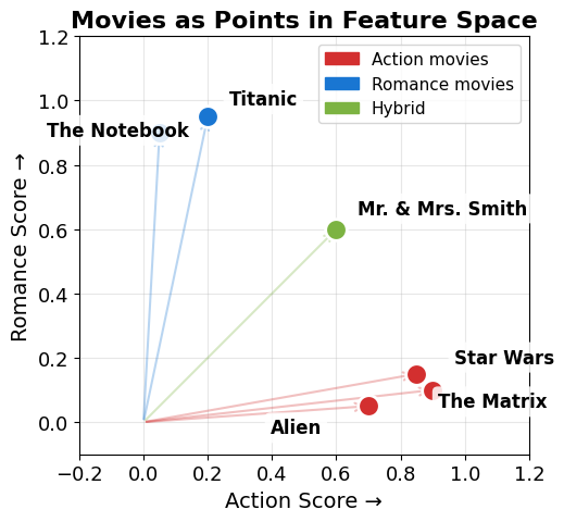
Similar movies are CLOSE in this space. That's the whole idea.
Source
# Same six movies, now with a 3rd axis (Sci-Fi). Action movies separate by how much sci-fi they add.
# Labels use proj_transform + 2-D pixel offsets so close pairs (Titanic/Notebook, Star Wars/Matrix)
# can be placed precisely in screen space — 3-D label offsets are unreliable.
from mpl_toolkits.mplot3d import proj3d

movies_3d = {
    'Star Wars':        (0.90, 0.10, 0.80),
    'The Matrix':       (0.85, 0.15, 0.90),
    'Alien':            (0.70, 0.05, 0.85),
    'Titanic':          (0.20, 0.95, 0.00),
    'The Notebook':     (0.05, 0.90, 0.00),
    'Mr. & Mrs. Smith': (0.60, 0.60, 0.10),
}
colors3d = {'Star Wars': '#d32f2f', 'The Matrix': '#d32f2f', 'Alien': '#d32f2f',
            'Titanic': '#1976d2', 'The Notebook': '#1976d2', 'Mr. & Mrs. Smith': '#7cb342'}

# Per-label pixel offsets (dx, dy) from the projected dot position, plus alignment.
label_style = {
    #             (dx,  dy,  ha,     va)
    'Star Wars':        (10,  16, 'left',  'bottom'),
    'The Matrix':       (12, -18, 'left',  'top'),
    'Alien':            (-12, 16, 'right', 'bottom'),
    'Titanic':          (12,  -3, 'left',  'center'),
    'The Notebook':     (-12, -3, 'right', 'center'),
    'Mr. & Mrs. Smith': (12,   0, 'left',  'center'),
}

fig = plt.figure(figsize=(8.5, 6.0))
ax = fig.add_subplot(111, projection='3d')

for name, (x, y, z) in movies_3d.items():
    ax.scatter(x, y, z, s=220, c=colors3d[name], edgecolors='white', linewidth=2)
    ax.plot([x, x], [y, y], [0, z], color=colors3d[name], alpha=0.30, lw=1)

ax.view_init(elev=22, azim=-55)
ax.set_xlim(0, 1); ax.set_ylim(0, 1); ax.set_zlim(0, 1)

ax.set_xlabel('Action ' + chr(0x2192),  fontsize=12, labelpad=10, fontweight='bold')
ax.set_ylabel('Romance ' + chr(0x2192), fontsize=12, labelpad=10, fontweight='bold')
ax.set_zlabel('')
ax.set_title('Movies as Points in 3D Feature Space', fontweight='bold', pad=14)

# Draw once so the projection matrix is up to date, then add screen-space labels.
fig.canvas.draw()
for name, (x, y, z) in movies_3d.items():
    x2, y2, _ = proj3d.proj_transform(x, y, z, ax.get_proj())
    dx, dy, ha, va = label_style[name]
    ax.annotate(name, xy=(x2, y2), xycoords='data',
                xytext=(dx, dy), textcoords='offset points',
                fontsize=10, fontweight='bold', ha=ha, va=va,
                bbox=dict(boxstyle='round,pad=0.2', facecolor='white',
                          edgecolor='none', alpha=0.7))

fig.text(0.79, 0.52, 'Sci-Fi ' + chr(0x2192), fontsize=12, fontweight='bold', rotation=90,
         va='center', ha='left')
fig.subplots_adjust(left=0.02, right=0.82, top=0.92, bottom=0.04)
plt.show()
print('Action movies (red) cluster at high Action + Sci-Fi; romances (blue) sit on the floor (Sci-Fi = 0).')
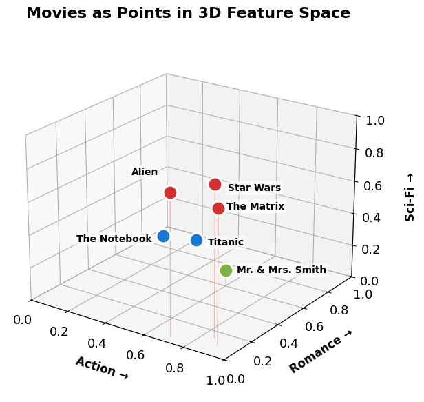
Action movies (red) cluster at high Action + Sci-Fi; romances (blue) sit on the floor (Sci-Fi = 0).
From 2 features to 3 … to hundreds
Two numbers → a point in 2D. Add a third feature (Sci-Fi) and the same movies spread out in 3D.
The math never cares how many axes there are — a movie with 20 genres is just a point in 20-dimensional space. We simply can’t draw past three.
Building the Item-Feature Matrix
Each movie has genres. We turn them into a binary vector (one-hot encoding).
Source
# One-hot encode genres
genre_matrix = movies['genres'].str.get_dummies(sep='|')
genre_matrix.index = movies['movieId']

# Visualize a slice
sample_ids = movies.head(15)['movieId'].values
sample_titles = movies.head(15)['title'].str[:25].values
sample_genres = genre_matrix.loc[sample_ids]

fig, ax = plt.subplots(figsize=(10, 4.8))
sns.heatmap(sample_genres, cmap=['#e0e0e0', '#1976d2'], cbar=False,
            linewidths=0.5, linecolor='white', ax=ax,
            yticklabels=sample_titles)
ax.set_title('Item-Feature Matrix (genres as binary vectors)', fontweight='bold')
ax.set_xlabel('Genre')
ax.tick_params(axis='x', rotation=45)
plt.tight_layout()
plt.show()

print(f'Each movie is a vector with {genre_matrix.shape[1]} dimensions (one per genre).')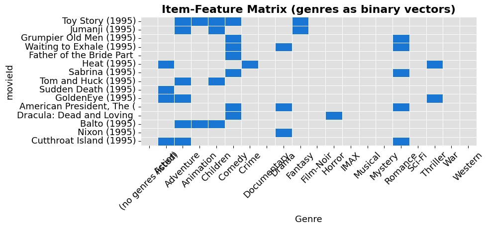
Each movie is a vector with 20 dimensions (one per genre).
Seeing all of them at once
We can’t plot 20 genre-dimensions, so we project every movie down to 2D with PCA — neighbours in this picture really are similar in genre space.
Source
pca = PCA(n_components=2)
movies_2d = pca.fit_transform(genre_matrix)

movies['primary_genre'] = movies['genres'].str.split('|').str[0]
top_genres = movies['primary_genre'].value_counts().head(6).index

genre_colors = {'Drama':'#1976d2', 'Comedy':'#388e3c', 'Action':'#d32f2f',
                'Horror':'#7b1fa2', 'Thriller':'#f57c00', 'Romance':'#e91e63'}

fig, ax = plt.subplots(figsize=(9.5, 5.5))
for genre in top_genres:
    mask = movies['primary_genre'] == genre
    ax.scatter(movies_2d[mask, 0], movies_2d[mask, 1],
               label=genre, alpha=0.35, s=20,
               color=genre_colors.get(genre, '#999'))

# Label some well-known movies
for name in ['Toy Story', 'Matrix', 'Titanic', 'Godfather', 'Pulp Fiction', 'Jurassic Park', 'Forrest Gump']:
    match = movies[movies['title'].str.contains(name, case=False)]
    if len(match) > 0:
        i = match.index[0]
        ax.annotate(match['title'].values[0][:25], (movies_2d[i, 0], movies_2d[i, 1]),
                    textcoords='offset points', xytext=(10, 10),
                    fontsize=9, fontweight='bold',
                    bbox=dict(boxstyle='round,pad=0.2', facecolor='yellow', alpha=0.85))
        ax.scatter(movies_2d[i, 0], movies_2d[i, 1], s=80, color='black', zorder=5)

ax.set_title('All Movies Projected to 2D (PCA on genre vectors)', fontweight='bold')
ax.legend(fontsize=11, markerscale=2)
ax.set_xlabel(f'PC1 ({pca.explained_variance_ratio_[0]:.0%} variance)')
ax.set_ylabel(f'PC2 ({pca.explained_variance_ratio_[1]:.0%} variance)')
plt.tight_layout()
plt.show()
print('Similar genre profiles → close in space. But 2D is a rough approximation of 20 dimensions.')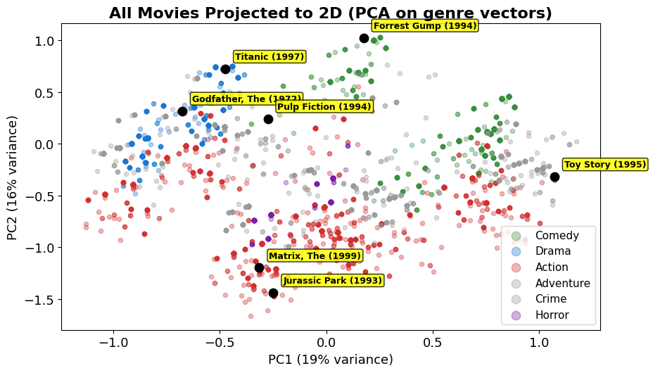
Similar genre profiles → close in space. But 2D is a rough approximation of 20 dimensions.
Beyond genres: richer movie vectors
We started with just genre flags (~20 dimensions). Real recommenders add whatever signal helps:
| Source | Example features |
|---|---|
| Cast & crew | director, lead actors, composer, cinematographer |
| Plot keywords | “time travel”, “heist”, “based on true story” |
| Metadata | year, runtime, country, MPAA rating |
| User signals | tags, average rating, popularity |
Every new feature is another dimension of the same vector. Two movies sharing the same director or composer become close even if their genres differ — capturing the kind of “more of the same” that genres alone miss.
(More dimensions = more nuance, but also the curse of dimensionality. Watch for that in a few slides.)
Users are vectors too
Describe each user with the same feature axes as the items. Then a recommender is just: “find items whose vector points the same way as this user’s.”
A user vector can come from a questionnaire, the average of items they watched/clicked, or feature extraction over their history.
Source
# A made-up user-feature matrix: how strongly each user likes each genre (0-1),
# living in the SAME feature space as the items.
user_features = pd.DataFrame(
    {'Action':  [0.9, 0.1, 0.5, 0.8, 0.2],
     'Romance': [0.1, 0.9, 0.4, 0.0, 0.7],
     'Sci-Fi':  [0.8, 0.0, 0.3, 0.9, 0.1],
     'Comedy':  [0.2, 0.6, 0.8, 0.1, 0.9],
     'Horror':  [0.7, 0.0, 0.1, 0.6, 0.0]},
    index=['Alice', 'Bob', 'Carol', 'Dave', 'Erin'])

fig, ax = plt.subplots(figsize=(7.0, 3.8))
hm = sns.heatmap(user_features, annot=True, cmap='Blues', vmin=0, vmax=1,
            cbar_kws={'label': 'preference'}, linewidths=0.5, linecolor='white', ax=ax)
ax.set_title('User-Feature Matrix (same axes as the items)', fontweight='bold')
plt.setp(hm.get_yticklabels(), rotation=0)
plt.setp(hm.get_xticklabels(), rotation=0)
ax.set_xlabel('feature (genre)')
ax.set_ylabel('user')
plt.tight_layout()
plt.show()
print('Alice and Dave both love Action + Sci-Fi -> their vectors point the same way -> similar taste.')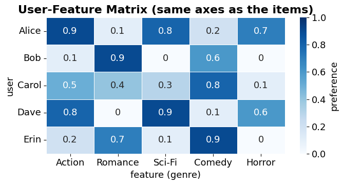
Alice and Dave both love Action + Sci-Fi -> their vectors point the same way -> similar taste.
Comparing Vectors: Dot Product
Multiply matching components, then sum — both as an algebraic recipe and a geometric identity:
Worked example. With and :
And the length (Euclidean norm, used in every formula below) of a vector:
Source
# Dot product as a projection: a . b = |a| * (length of b projected onto a)
fig, ax = plt.subplots(figsize=(7.5, 5.0))
a = np.array([1.0, 0.15])
b = np.array([0.55, 0.60])
a_hat = a / np.linalg.norm(a)
proj = np.dot(b, a_hat) * a_hat                 # vector projection of b onto a

ax.annotate('', xy=a, xytext=(0, 0), arrowprops=dict(arrowstyle='->', lw=3, color='#1976d2'))
ax.annotate('', xy=b, xytext=(0, 0), arrowprops=dict(arrowstyle='->', lw=3, color='#d32f2f'))
ax.annotate('', xy=proj, xytext=(0, 0), arrowprops=dict(arrowstyle='->', lw=4, color='#388e3c'))
ax.plot([b[0], proj[0]], [b[1], proj[1]], ls='--', color='gray', lw=1.5)   # drop line
ax.text(a[0] + 0.02, a[1] - 0.06, 'a', color='#1976d2', fontsize=16, fontweight='bold')
ax.text(b[0] + 0.02, b[1] + 0.02, 'b', color='#d32f2f', fontsize=16, fontweight='bold')
ax.text(proj[0] * 0.5, proj[1] * 0.5 - 0.09, 'projection of b onto a',
        color='#388e3c', fontsize=11, fontweight='bold')

ax.set_title(f'a · b = {np.dot(a, b):.2f}  =  |a| · |b| · cos(θ)', fontweight='bold')
ax.set_xlim(-0.1, 1.2)
ax.set_ylim(-0.1, 0.85)
ax.set_aspect('equal')
ax.grid(True, alpha=0.3)
ax.spines[['top', 'right']].set_visible(False)
plt.tight_layout()
plt.show()
print('A longer b gives a bigger dot product at the same angle. Cosine divides by both lengths, so only the angle survives.')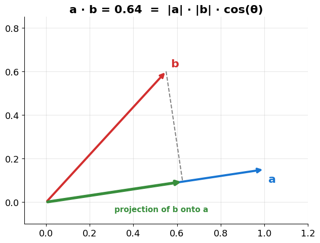
A longer b gives a bigger dot product at the same angle. Cosine divides by both lengths, so only the angle survives.
Cosine Similarity: dot product, length removed
Take the dot-product identity and isolate the angle — move everything except to the right side:
So cosine similarity = dot product after normalising both vectors to length 1 — it ignores magnitude, only the angle remains.
Source
# One clean picture: the angle theta between two vectors IS the cosine similarity.
fig, ax = plt.subplots(figsize=(6.0, 5.5))
a = np.array([0.90, 0.25])
b = np.array([0.45, 0.75])
cos = np.dot(a, b) / (np.linalg.norm(a) * np.linalg.norm(b))
theta = np.degrees(np.arccos(cos))

ax.annotate('', xy=a, xytext=(0, 0), arrowprops=dict(arrowstyle='->', lw=3, color='#1976d2'))
ax.annotate('', xy=b, xytext=(0, 0), arrowprops=dict(arrowstyle='->', lw=3, color='#d32f2f'))
arc = mpatches.Arc((0, 0), 0.5, 0.5, angle=0,
                   theta1=np.degrees(np.arctan2(a[1], a[0])),
                   theta2=np.degrees(np.arctan2(b[1], b[0])), color='#388e3c', lw=2.5)
ax.add_patch(arc)
ax.text(0.30, 0.22, f'θ = {theta:.0f}°', fontsize=15, color='#388e3c', fontweight='bold')
ax.text(a[0] + 0.02, a[1] - 0.03, 'a', fontsize=16, fontweight='bold', color='#1976d2')
ax.text(b[0] + 0.02, b[1] + 0.02, 'b', fontsize=16, fontweight='bold', color='#d32f2f')
ax.text(0.42, 0.95, f'cos(θ) = {cos:.2f}', fontsize=16, fontweight='bold',
        bbox=dict(boxstyle='round,pad=0.4', facecolor='#fff9c4'))

ax.set_xlim(-0.1, 1.05)
ax.set_ylim(-0.1, 1.05)
ax.set_aspect('equal')
ax.grid(True, alpha=0.3)
ax.axhline(0, color='gray', lw=0.5)
ax.axvline(0, color='gray', lw=0.5)
ax.spines[['top', 'right']].set_visible(False)
ax.set_title('Cosine similarity = cosine of the angle θ', fontweight='bold')
plt.tight_layout()
plt.show()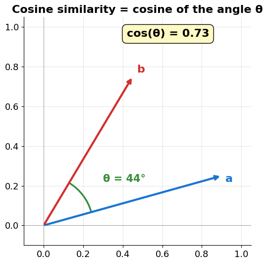
What the number actually means
Same reference vector, swept from 0° to 180°. Cosine starts at 1 (identical direction), is 0 at a right angle, and reaches −1 when the vectors point opposite ways.
Source
fig, (ax1, ax2) = plt.subplots(1, 2, figsize=(11, 4.5))
cmap = plt.cm.RdYlGn
angles = [0, 30, 60, 90, 120, 150, 180]

# Left: a fan of test vectors at increasing angles from the x-axis
for ang in angles:
    r = np.radians(ang)
    v = np.array([np.cos(r), np.sin(r)])
    c = cmap((np.cos(r) + 1) / 2)            # map cos in [-1, 1] -> colour in [0, 1]
    ax1.annotate('', xy=v, xytext=(0, 0), arrowprops=dict(arrowstyle='->', lw=2.5, color=c))
    ax1.text(v[0] * 1.13, v[1] * 1.13, f'{ang}°', ha='center', va='center', fontsize=11, fontweight='bold')
ax1.add_patch(plt.Circle((0, 0), 1, fill=False, color='gray', alpha=0.3))
ax1.set_xlim(-1.3, 1.3)
ax1.set_ylim(-0.3, 1.3)
ax1.set_aspect('equal')
ax1.axis('off')
ax1.set_title('Test vectors at increasing angles', fontweight='bold')

# Right: cosine as a function of the angle
deg = np.linspace(0, 180, 200)
ax2.plot(deg, np.cos(np.radians(deg)), color='#1976d2', lw=3)
for ang in angles:
    ax2.scatter(ang, np.cos(np.radians(ang)), s=80, zorder=5, edgecolors='black',
                color=cmap((np.cos(np.radians(ang)) + 1) / 2))
ax2.axhline(0, color='gray', lw=0.8, ls='--')
ax2.set_xticks(angles)
ax2.set_ylim(-1.25, 1.18)   # headroom below the curve so 'opposite' clears the line
ax2.set_xlabel('angle between vectors (degrees)')
ax2.set_ylabel('cosine similarity')
ax2.set_title('cos(θ):  1 → 0 → −1', fontweight='bold')
ax2.spines[['top', 'right']].set_visible(False)
# Keep each label off the blue curve: identical sits below-right of (0,1),
# orthogonal above-right of (90,0), opposite below-left of (180,-1).
ax2.annotate('identical',  (0, 1),    textcoords='offset points', xytext=(10, -16), ha='left',  va='top',    fontsize=10, color='#388e3c')
ax2.annotate('orthogonal', (90, 0),   textcoords='offset points', xytext=(8, 12),   ha='left',  va='bottom', fontsize=10, color='#f57c00')
ax2.annotate('opposite',   (180, -1), textcoords='offset points', xytext=(-8, -12), ha='right', va='top',    fontsize=10, color='#d32f2f')
plt.tight_layout()
plt.show()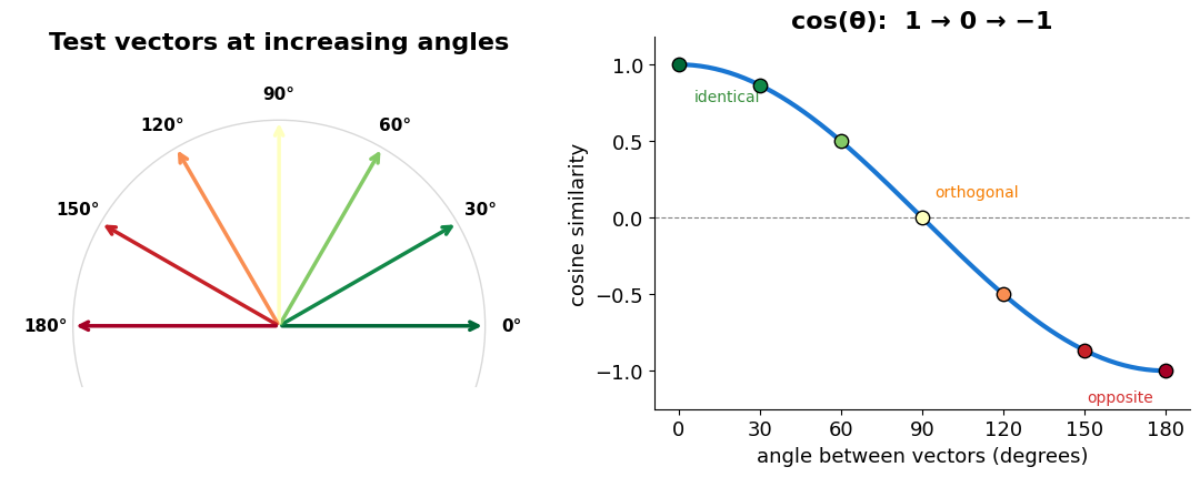
Cosine on movie-like vectors: three cases
Source
# Three "textbook" cases -- pick vectors so the cosine actually hits the labeled values.
# a is the same reference movie in every case; b is rotated to hit cos = 0.95, 0.50, 0.00,
# and each b is a real movie whose similarity to the reference matches that angle.
fig, axes = plt.subplots(1, 3, figsize=(11, 3.8))

a = np.array([1.0, 0.0])
ref_movie = 'Star Wars'                        # vector a -- same reference in all three panels
target_cos = [0.95, 0.50, 0.00]
# (case label, colour, movie for b, b-label offset in points, b-label h-align)
case_meta = [
    ('Very Similar',     '#388e3c', 'The Matrix',       (-4, 12), 'right'),
    ('Somewhat Similar', '#f57c00', 'Mr. & Mrs. Smith', (0, 12),  'center'),
    ('Not Similar',      '#d32f2f', 'The Notebook',     (8, 2),   'left'),
]

for ax, target, (label, color, b_movie, b_off, b_ha) in zip(axes, target_cos, case_meta):
    theta = np.arccos(target)
    b = np.array([np.cos(theta), np.sin(theta)])
    cos = float(np.dot(a, b))   # equals target by construction

    ax.annotate('', xy=a, xytext=(0, 0), arrowprops=dict(arrowstyle='->', lw=3, color='#1976d2'))
    ax.annotate('', xy=b, xytext=(0, 0), arrowprops=dict(arrowstyle='->', lw=3, color='#d32f2f'))

    angle_a = np.degrees(np.arctan2(a[1], a[0]))
    angle_b = np.degrees(np.arctan2(b[1], b[0]))
    arc = mpatches.Arc((0, 0), 0.4, 0.4, angle=0,
                       theta1=min(angle_a, angle_b), theta2=max(angle_a, angle_b),
                       color=color, lw=2)
    ax.add_patch(arc)
    ax.text(0.25, 0.10, f'angle = {np.degrees(theta):.0f}°',
            color=color, fontsize=11, fontweight='bold')

    # Label the arrows with real movie names instead of 'a' / 'b'.
    ax.annotate(ref_movie, xy=a, xytext=(-4, -12), textcoords='offset points',
                ha='right', va='top', fontsize=9.5, fontweight='bold', color='#1976d2')
    ax.annotate(b_movie, xy=b, xytext=b_off, textcoords='offset points',
                ha=b_ha, va='bottom', fontsize=9.5, fontweight='bold', color='#d32f2f')
    ax.set_title(f'{label}\ncos = {cos:.2f}', fontweight='bold', color=color)
    ax.set_xlim(-0.15, 1.15); ax.set_ylim(-0.28, 1.18); ax.set_aspect('equal')
    ax.grid(True, alpha=0.3)
    ax.axhline(y=0, color='gray', lw=0.5)
    ax.axvline(x=0, color='gray', lw=0.5)
    ax.spines[['top', 'right']].set_visible(False)

plt.suptitle('Cosine Similarity = angle between vectors', fontsize=15, y=1.02)
plt.tight_layout()
plt.show()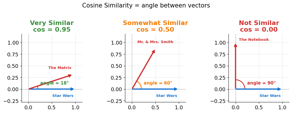
Euclidean Distance = the straight-line gap
Algebraic form (works in any number of dimensions):
Forget angles — just measure the distance between the two points.
Small distance = similar.
(As a similarity score we often use , since closer should mean “more similar”.)
Source
# Euclidean distance is just Pythagoras on the difference vector.
fig, ax = plt.subplots(figsize=(6.5, 5.5))
a = np.array([0.30, 0.70])
b = np.array([0.85, 0.25])
d = np.linalg.norm(a - b)

ax.scatter(*a, s=200, color='#1976d2', zorder=5, edgecolors='white', linewidth=2)
ax.scatter(*b, s=200, color='#d32f2f', zorder=5, edgecolors='white', linewidth=2)
ax.plot([a[0], b[0]], [a[1], b[1]], color='#7b1fa2', lw=3)              # hypotenuse = distance
ax.plot([a[0], b[0]], [a[1], a[1]], ls='--', color='gray', lw=1.5)     # horizontal leg
ax.plot([b[0], b[0]], [a[1], b[1]], ls='--', color='gray', lw=1.5)     # vertical leg
ax.text((a[0] + b[0]) / 2 - 0.02, (a[1] + b[1]) / 2 + 0.04, f'd = {d:.2f}',
        color='#7b1fa2', fontsize=15, fontweight='bold')
ax.text((a[0] + b[0]) / 2, a[1] - 0.06, f'Δx = {abs(a[0] - b[0]):.2f}', color='gray', fontsize=11, ha='center')
ax.text(b[0] + 0.01, (a[1] + b[1]) / 2, f'Δy = {abs(a[1] - b[1]):.2f}', color='gray', fontsize=11)
ax.text(a[0] - 0.03, a[1] + 0.03, 'a', color='#1976d2', fontsize=16, fontweight='bold')
ax.text(b[0] + 0.05, b[1] - 0.02, 'b', color='#d32f2f', fontsize=16, fontweight='bold')

ax.set_title('Geometric (2D) form:  √(Δx² + Δy²)', fontweight='bold')
ax.set_xlim(0, 1.05)
ax.set_ylim(0, 1.05)
ax.set_aspect('equal')
ax.grid(True, alpha=0.3)
ax.spines[['top', 'right']].set_visible(False)
plt.tight_layout()
plt.show()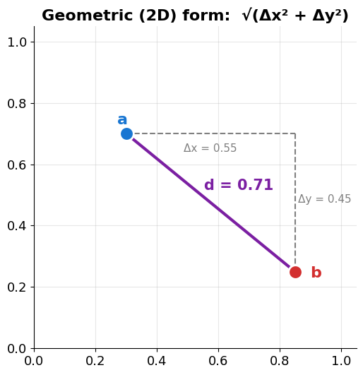
Manhattan Distance = the city-block path
Instead of the diagonal hypotenuse, sum the absolute differences — as if you can only walk along the grid, N/S or E/W. Manhattan ≥ Euclidean always (the diagonal is shorter than the L-shape).
In high-dimensional, sparse vectors (where most coordinates are zero) L1 is often the more robust choice for nearest-neighbour search — no squaring means fewer dimensions dominate the score.
Source
# Same two points as the Euclidean slide — but here we walk the grid (no diagonal shortcut).
fig, (ax1, ax2) = plt.subplots(1, 2, figsize=(10, 4.4))

a = np.array([0.30, 0.70])
b = np.array([0.85, 0.25])
euc = np.linalg.norm(a - b)
man = np.abs(a - b).sum()

# (1) Euclidean — the diagonal, for reference.
ax1.scatter(*a, s=200, color='#1976d2', zorder=5, edgecolors='white', linewidth=2)
ax1.scatter(*b, s=200, color='#d32f2f', zorder=5, edgecolors='white', linewidth=2)
ax1.plot([a[0], b[0]], [a[1], b[1]], color='#7b1fa2', lw=3, label=f'Euclidean = {euc:.2f}')
ax1.text(a[0] - 0.06, a[1] + 0.04, 'a', color='#1976d2', fontsize=16, fontweight='bold')
ax1.text(b[0] + 0.04, b[1] + 0.04, 'b', color='#d32f2f', fontsize=16, fontweight='bold')
ax1.set_title('Euclidean: the diagonal', fontweight='bold')
ax1.set_xlim(0, 1.05); ax1.set_ylim(0, 1.05); ax1.set_aspect('equal')
ax1.grid(True, alpha=0.3); ax1.spines[['top', 'right']].set_visible(False)
ax1.legend(loc='upper right')

# (2) Manhattan — two axis-aligned legs whose lengths add up to |Δx| + |Δy|.
ax2.scatter(*a, s=200, color='#1976d2', zorder=5, edgecolors='white', linewidth=2)
ax2.scatter(*b, s=200, color='#d32f2f', zorder=5, edgecolors='white', linewidth=2)
ax2.plot([a[0], b[0]], [a[1], a[1]], color='#f57c00', lw=3)
ax2.plot([b[0], b[0]], [a[1], b[1]], color='#f57c00', lw=3, label=f'Manhattan = {man:.2f}')
ax2.text(a[0] - 0.06, a[1] + 0.04, 'a', color='#1976d2', fontsize=16, fontweight='bold')
ax2.text(b[0] + 0.04, b[1] + 0.04, 'b', color='#d32f2f', fontsize=16, fontweight='bold')
ax2.text((a[0] + b[0]) / 2, a[1] + 0.03, f'|Δx| = {abs(a[0] - b[0]):.2f}',
         color='gray', ha='center', fontsize=11)
ax2.text(b[0] + 0.02, (a[1] + b[1]) / 2, f'|Δy| = {abs(a[1] - b[1]):.2f}',
         color='gray', fontsize=11)
ax2.set_title('Manhattan: sum of axis-aligned steps', fontweight='bold')
ax2.set_xlim(0, 1.05); ax2.set_ylim(0, 1.05); ax2.set_aspect('equal')
ax2.grid(True, alpha=0.3); ax2.spines[['top', 'right']].set_visible(False)
ax2.legend(loc='upper right')

plt.suptitle(f'Same two points — Manhattan ({man:.2f}) ≥ Euclidean ({euc:.2f})',
             fontsize=14, fontweight='bold', y=1.02)
plt.tight_layout()
plt.show()
print('Manhattan = L1 norm of (a - b); Euclidean = L2. In high-D, L1 is often the more robust choice.')
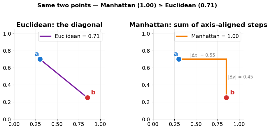
Manhattan = L1 norm of (a - b); Euclidean = L2. In high-D, L1 is often the more robust choice.
Summary: Cosine vs. Euclidean vs. Dot Product vs. Manhattan
Same three vectors (a, b1, and b2 = 2·b1), four different verdicts on “which of b1 or b2 is closer to a?”
Source
# Setup: a is the QUERY (e.g. a movie the user just liked); b1, b2 are two CANDIDATES
# in the catalog. The recommender must rank them. Each metric scores (a, candidate)
# and the candidate with the better score is shown first. b2 = 2*b1 -- same DIRECTION
# as b1 but twice as LONG (think: more tags, more ratings, longer description).
fig, axes = plt.subplots(2, 2, figsize=(10, 7.0))

a  = np.array([0.8, 0.3])   # query
b1 = np.array([0.7, 0.4])   # candidate 1
b2 = 2 * b1                 # candidate 2 -- same direction, twice as long


def draw_vectors(ax, title, extras=None):
    ax.annotate('', xy=a,  xytext=(0, 0), arrowprops=dict(arrowstyle='->', lw=3, color='#1976d2'))
    ax.annotate('', xy=b1, xytext=(0, 0), arrowprops=dict(arrowstyle='->', lw=3, color='#d32f2f'))
    ax.annotate('', xy=b2, xytext=(0, 0), arrowprops=dict(arrowstyle='->', lw=3, color='#388e3c'))
    ax.text(a[0]  + 0.03, a[1] - 0.04, 'a  (query)',
            color='#1976d2', fontweight='bold', fontsize=11)
    # b1 label sits up-left of its arrowhead so it doesn't land on the collinear b2 arrow.
    ax.text(b1[0] - 0.05, b1[1] + 0.11, 'b1  (cand. 1)',
            color='#d32f2f', fontweight='bold', fontsize=11, ha='right', va='bottom')
    ax.text(b2[0] + 0.03, b2[1],       'b2  (cand. 2, = 2*b1)',
            color='#388e3c', fontweight='bold', fontsize=11)
    if extras: extras(ax)
    ax.set_title(title, fontweight='bold', fontsize=11, loc='center')
    ax.set_xlim(-0.1, 1.95); ax.set_ylim(-0.1, 1.0); ax.set_aspect('equal')
    ax.grid(True, alpha=0.3); ax.spines[['top', 'right']].set_visible(False)


cos1 = np.dot(a, b1) / (np.linalg.norm(a) * np.linalg.norm(b1))
cos2 = np.dot(a, b2) / (np.linalg.norm(a) * np.linalg.norm(b2))
draw_vectors(axes[0, 0],
             f'COSINE   (higher = better)\n'
             f'b1: {cos1:.2f}    b2: {cos2:.2f}    ->   TIE  (length ignored)')

dot1 = np.dot(a, b1); dot2 = np.dot(a, b2)
draw_vectors(axes[0, 1],
             f'DOT PRODUCT   (higher = better)\n'
             f'b1: {dot1:.2f}    b2: {dot2:.2f}    ->   ranks b2 first  (length rewarded)')

euc1 = np.linalg.norm(a - b1); euc2 = np.linalg.norm(a - b2)
def euc_extras(ax):
    ax.plot([a[0], b1[0]], [a[1], b1[1]], '--', color='#d32f2f', lw=1.5)
    ax.plot([a[0], b2[0]], [a[1], b2[1]], '--', color='#388e3c', lw=1.5)
draw_vectors(axes[1, 0],
             f'EUCLIDEAN  (L2 distance, LOWER = better)\n'
             f'b1: {euc1:.2f}    b2: {euc2:.2f}    ->   ranks b1 first',
             extras=euc_extras)

man1 = np.abs(a - b1).sum(); man2 = np.abs(a - b2).sum()
def man_extras(ax):
    for b_, c_ in [(b1, '#d32f2f'), (b2, '#388e3c')]:
        ax.plot([a[0], b_[0]], [a[1], a[1]], color=c_, ls=':', lw=1.5)
        ax.plot([b_[0], b_[0]], [a[1], b_[1]], color=c_, ls=':', lw=1.5)
draw_vectors(axes[1, 1],
             f'MANHATTAN  (L1 distance, LOWER = better)\n'
             f'b1: {man1:.2f}    b2: {man2:.2f}    ->   ranks b1 first  (same as L2)',
             extras=man_extras)

plt.suptitle('Which candidate should the recommender show next?\n'
             'Same query a, same two candidates b1 and b2 -- different metrics, different rankings.',
             fontsize=13, y=0.99, fontweight='bold')
fig.subplots_adjust(left=0.06, right=0.97, top=0.82, bottom=0.05, wspace=0.30, hspace=0.45)
plt.show()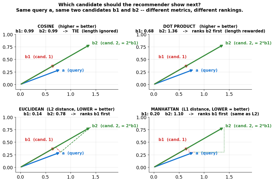
When to use which measure
| Measure | Best for | Why |
|---|---|---|
| Cosine | text, tags, bag-of-words — anywhere lengths vary | only angle counts, so a 10-word and a 1000-word doc compare fairly |
| Dot product | recommender scores (e.g. matrix factorisation) | rewards both alignment and confidence/length |
| Euclidean (L2) | dense vectors where magnitude is meaningful | straight-line gap; squaring amplifies large differences |
| Manhattan (L1) | high-dim sparse, non-learned vectors (raw TF-IDF, counts) | no squaring, so fewer single dims dominate — a rule of thumb (Aggarwal et al. 2001), not a law |
Pick the metric by where the vectors came from — not by their dimensionality:
Learned embeddings (sentence transformers, …) → use the metric they were trained with, almost always cosine / dot — at 384 or 4096 dims. Don’t switch to L1 just because it’s high-dimensional.
Sparse, non-learned vectors (TF-IDF, counts) → cosine; L1 is worth a try in very high dimensions.
Normalise and the distinction often vanishes: for unit vectors , so cosine, dot product, and Euclidean rank neighbours in the identical order.
The Curse of Dimensionality
Genre vectors live in ~20 dimensions; real feature vectors can have thousands. As dimensionality grows, something counter-intuitive happens to distance.
The phenomenon. Beyer et al. (1999) proved that for a wide class of distributions, as the ratio of the farthest to the nearest neighbour of a query point tends to 1. In very high dimensions every point is roughly the same distance from every other point — so “nearest neighbour” loses its meaning.
Geometric intuition. Fix the unit cube . Two things happen as grows:
The inscribed unit ball’s volume shrinks toward 0 — almost all the cube’s mass sits in the corners, not near the centre.
Almost all of a -ball’s volume concentrates in a thin shell at the boundary, so two random points have nearly the same radius and their pairwise distances bunch into a narrow band.
Why cosine survives better — with caveats. Cosine isn’t immune: for dense random vectors in high , every pair becomes nearly orthogonal (cos 0) and the curse hits it too. But the vectors used in content-based recommending — TF-IDF, tag indicators, one-hot features — are sparse: similarity is driven by the handful of dimensions where both vectors are non-zero. That handful carries the signal; the many shared zeros are silent (they neither add to the numerator nor distort the angle), whereas in Euclidean distance every dimension contributes a small 0−ε term and the noise piles up. Discarding magnitude also removes one source of variation that carries no meaning for count-style vectors.
📚 Sources: Beyer, Goldstein, Ramakrishnan & Shaft (1999), When Is “Nearest Neighbor” Meaningful? (ICDT); Aggarwal, Hinneburg & Keim (2001), On the Surprising Behavior of Distance Metrics in High Dimensional Space.
Source
# Two panels show the same phenomenon from two angles:
# (1) the contrast (farthest − nearest)/nearest crashes toward 0 as d grows,
# (2) the distribution of pairwise distances piles into a narrow band — so "near" and "far"
#     become indistinguishable. No need for a 3-D scatter; the histogram tells the story.
rng = np.random.default_rng(0)

fig, (ax1, ax2) = plt.subplots(1, 2, figsize=(11, 4.4))

# (1) Distance contrast vs dimensionality.
dims = [2, 5, 10, 50, 100, 500, 1000]
contrast = []
for d in dims:
    X = rng.random((300, d))
    dist = np.linalg.norm(X[1:] - X[0], axis=1)
    contrast.append((dist.max() - dist.min()) / dist.min())
ax1.plot(dims, contrast, 'o-', color='#d32f2f', lw=2.5, markersize=10)
for d, c in zip(dims, contrast):
    ax1.annotate(f'{c:.2f}', (d, c), textcoords='offset points', xytext=(8, 6), fontsize=9)
ax1.set_xscale('log')
ax1.set_xlabel('number of dimensions  d')
ax1.set_ylabel('(farthest − nearest) / nearest')
ax1.set_title('Distance contrast collapses', fontweight='bold')
ax1.axhline(0, color='gray', ls='--', alpha=0.5)
ax1.spines[['top', 'right']].set_visible(False)

# (2) Pairwise distance distribution at d = 2 → 10 → 100 → 1000.
# Scale by √d so curves overlap and we can visually compare *widths* (spread shrinks).
for d, color, label in [(2, '#1976d2', '2-D'), (10, '#388e3c', '10-D'),
                        (100, '#f57c00', '100-D'), (1000, '#7b1fa2', '1000-D')]:
    Y = rng.random((400, d))
    dd = np.linalg.norm(Y[:200] - Y[200:], axis=1) / np.sqrt(d)
    ax2.hist(dd, bins=35, alpha=0.55, color=color, label=label, density=True)
ax2.set_xlabel('pairwise distance (scaled by √d)')
ax2.set_ylabel('density')
ax2.set_title('Higher d → distances pile into a narrow band', fontweight='bold')
ax2.legend(loc='upper right')
ax2.spines[['top', 'right']].set_visible(False)

plt.tight_layout()
plt.show()
print('At d = 1000, every pair of points is essentially the same distance apart — '
      '"nearest neighbour" no longer means anything.')
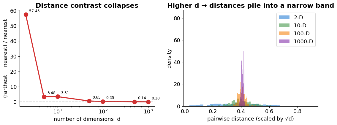
At d = 1000, every pair of points is essentially the same distance apart — "nearest neighbour" no longer means anything.
Beyond hand-crafted features
So far every feature has been hand-designed — genres, plus the richer columns we sketched (cast, keywords, decade, popularity). Someone has to choose them, label them, and keep them updated. That does not scale.
The real power: turn any data into a vector automatically — then reuse the exact same similarity tools.
| Data | How it becomes a vector |
|---|---|
| Text | bag-of-words / TF-IDF → word & sentence embeddings |
| Images | pixel features → CNN embeddings |
| Tabular | the columns already are the vector |
| Anything | a learned embedding model |
Once everything is a vector, similarity is similarity.
Source
# Schematic: three very different data types embed into ONE shared n-D space.
# Each modality has its own arrow INTO the embedding model; one arrow comes OUT
# of the model and points into the shared vector space.
fig, ax = plt.subplots(figsize=(10, 5))
ax.set_xlim(0, 1)
ax.set_ylim(0, 1)
ax.axis('off')

# Three input sources (left column).
sources = [
    ('"A space western about\na rogue hero…"   (text)', 0.02, 0.78, '#1976d2'),
    ('[ image ]  movie poster   (image)',              0.02, 0.50, '#388e3c'),
    ('Action=1, Sci-Fi=1, …   (table)',                0.02, 0.22, '#f57c00'),
]
for txt, x, y, c in sources:
    ax.text(x, y, txt, fontsize=11, va='center', ha='left',
            bbox=dict(boxstyle='round,pad=0.4', facecolor='white', edgecolor=c, lw=2))

# Embedding model box — single shared transformer.
box_x, box_y, box_w, box_h = 0.41, 0.40, 0.16, 0.20
ax.add_patch(mpatches.FancyBboxPatch((box_x, box_y), box_w, box_h, boxstyle='round,pad=0.02',
                                     facecolor='#f5f5f5', edgecolor='gray', lw=1.8))
ax.text(box_x + box_w / 2, box_y + box_h / 2, 'embedding\nmodel',
        fontsize=11, style='italic', color='dimgray', ha='center', va='center')

# Three arrows: each source -> LEFT edge of the box (so they clearly enter the model).
box_left = box_x
for _, x, y, c in sources:
    ax.annotate('', xy=(box_left, box_y + box_h / 2),
                xytext=(x + 0.32, y),
                arrowprops=dict(arrowstyle='->', color=c, lw=2.2, alpha=0.85))

# One arrow OUT of the box -> into the shared vector space.
ax.annotate('', xy=(0.66, box_y + box_h / 2),
            xytext=(box_x + box_w, box_y + box_h / 2),
            arrowprops=dict(arrowstyle='->', color='#7b1fa2', lw=2.5))

# Shared vector space — dashed-purple frame, scatter of points.
ax.add_patch(mpatches.FancyBboxPatch((0.66, 0.22), 0.32, 0.66, boxstyle='round,pad=0.01',
                                     facecolor='none', edgecolor='#7b1fa2', lw=2, ls='--'))
ax.text(0.82, 0.92, 'ONE shared n-D vector space', fontsize=12, fontweight='bold',
        color='#7b1fa2', ha='center')

pts = np.array([[0.74, 0.62], [0.78, 0.51], [0.88, 0.32], [0.71, 0.40], [0.92, 0.66]])
cols = ['#1976d2', '#388e3c', '#f57c00', '#1976d2', '#388e3c']
ax.scatter(pts[:, 0], pts[:, 1], s=180, c=cols, edgecolors='white', linewidth=2, zorder=4)

# Example vector right under the title.
ax.text(0.82, 0.82, 'one such vector  (length = 300)', fontsize=9, color='gray', ha='center')
ax.text(0.82, 0.76, '[ 0.32, -0.11,  0.74,  0.05, -0.42,  …,  0.07 ]',
        fontsize=10, color='#1976d2', family='monospace', ha='center',
        bbox=dict(boxstyle='round,pad=0.3', facecolor='white', edgecolor='#1976d2', lw=1))

# Caption sits BELOW the dashed frame.
ax.text(0.82, 0.12, 'every source → same dimensionality\n'
                    'so cosine / dot-product work across modalities',
        fontsize=10, color='#7b1fa2', ha='center', style='italic')

plt.tight_layout()
plt.show()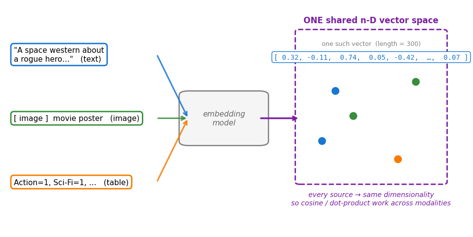
Step 1: Bag-of-Words — count the words, drop the order
The simplest way to turn text into a vector: pick a vocabulary, then for every document count how often each vocabulary word appears.
| document | space | rebels | empire | romance | iceberg |
|---|---|---|---|---|---|
| “space rebels fight an evil empire” | 1 | 1 | 1 | 0 | 0 |
| “a romance about a doomed ocean liner that hits an iceberg” | 0 | 0 | 0 | 1 | 1 |
Every row is now a vector in vocabulary space — and cosine similarity works exactly as before.
Catch: “the”, “a”, “movie” dominate every row → cosine is mostly noise. We need to down-weight common words ⤵
TF-IDF: turning text into vectors
TF-IDF = Term Frequency × Inverse Document Frequency. Bag-of-words just counts words; TF-IDF weights each count by how informative the word is.
df(t) is the document frequency — how many of the N documents contain t at least once.
Word in every doc → df = N → idf = log 1 = 0 (worthless).
Word in one doc → df = 1 → idf = log N (most distinctive).
Then two documents are compared with the same cosine similarity as before.
Practical note: smoothed idf. scikit-learn (and most modern implementations) use a smoothed variant:
The +1 in numerator and denominator pretends there is one extra document containing every term — so an unseen term (df = 0) does not divide by zero, and the trailing +1 keeps even ubiquitous words from being fully zeroed out (they still get a small weight equal to their tf). Ranking behaviour is essentially the same; only the absolute weights differ. (We use the classical form above because it makes the intuition cleaner.)
Intuition: why “the” gets weight 0 and “wormhole” gets a huge one
Pick a tiny corpus of N = 5 movie blurbs. For any word t:
tf(t, d) — how often t appears in document d
df(t) — how many of the 5 documents contain t (its doc-frequency)
idf(t) = — big when t is rare, 0 when t is everywhere
| word | df | verdict | |
|---|---|---|---|
| the | 5 | log(1) = 0 | killed — appears everywhere, useless |
| romance | 2 | log(2.5) ≈ 0.92 | discriminating — pairs the love stories |
| wormhole | 1 | log(5) ≈ 1.61 | very informative — almost defines that doc |
So a word’s weight = how often it shows up here × how rare it is overall. Multiply, and informative words dominate the vector.
Source
# Five tiny movie blurbs and the words that drive their similarity.
# Left: each blurb's TOP weighted tokens (what makes that doc unique).
# Right: for the top-3 most-similar pairs, the SHARED words that actually create the score
#        -- so students see "why" Titanic ↔ The Notebook pair up (the word "romance"), etc.
from sklearn.feature_extraction.text import TfidfVectorizer

docs = {
    'Star Wars':    'space rebels fight an evil galactic empire with laser swords',
    'The Matrix':   'a hacker discovers reality is a simulation and fights machines',
    'Titanic':      'a romance aboard a doomed ocean liner that hits an iceberg',
    'The Notebook': 'a sweeping romance remembered by an old man still in love',
    'Interstellar': 'astronauts travel through space and a wormhole to save humanity',
}
titles = list(docs)
tfidf = TfidfVectorizer(stop_words='english')
X = tfidf.fit_transform(docs.values())
sim = cosine_similarity(X)
vocab = tfidf.get_feature_names_out()
W = X.toarray()

fig, (ax1, ax2) = plt.subplots(1, 2, figsize=(11.5, 4.8))

# (1) Top-3 tokens per document as horizontal bars (one panel of 5 small bar groups).
TOPK = 3
ypos = 0
for d_idx, title in enumerate(titles):
    weights = W[d_idx]
    top_ids = weights.argsort()[::-1][:TOPK]
    for r, j in enumerate(top_ids):
        ax1.barh(ypos, weights[j], color='#1976d2', alpha=0.85, edgecolor='white')
        ax1.text(weights[j] + 0.005, ypos, f' {vocab[j]}  ({weights[j]:.2f})',
                 va='center', fontsize=10)
        ypos += 1
    ax1.axhline(ypos - 0.5, color='gray', lw=0.5, alpha=0.4)
    ax1.text(-0.04, ypos - TOPK / 2 - 0.5, title, ha='right', va='center',
             fontsize=11, fontweight='bold')
    ypos += 0.6
ax1.set_xlim(0, 0.7)
ax1.set_xlabel('tf-idf weight (higher = more distinctive)')
ax1.set_title('Each blurb in 3 words: top tf-idf tokens', fontweight='bold')
ax1.set_yticks([])
ax1.spines[['top', 'right', 'left']].set_visible(False)
ax1.invert_yaxis()

# (2) Shared words driving the TOP 3 pairs. Contribution = tfidf(w,d1) * tfidf(w,d2).
pairs = []
for i in range(len(titles)):
    for j in range(i + 1, len(titles)):
        pairs.append((sim[i, j], i, j))
pairs.sort(reverse=True)
ypos = 0
for s, i, j in pairs[:3]:
    contrib = W[i] * W[j]
    nz = np.where(contrib > 1e-6)[0]
    nz = nz[np.argsort(contrib[nz])[::-1]]
    pair_label = f'{titles[i]}  ↔  {titles[j]}   (cos = {s:.2f})'
    for k_, idx in enumerate(nz):
        ax2.barh(ypos, contrib[idx], color='#388e3c', alpha=0.85, edgecolor='white')
        ax2.text(contrib[idx] + 0.003, ypos, f' {vocab[idx]}',
                 va='center', fontsize=10)
        ypos += 1
    if len(nz) == 0:
        ax2.text(0.005, ypos, '(no shared tokens above stop-word filter)',
                 color='gray', fontsize=10, fontstyle='italic')
        ypos += 1
    ax2.text(-0.005, ypos - max(len(nz), 1) / 2 - 0.5, pair_label, ha='right', va='center',
             fontsize=11, fontweight='bold')
    ax2.axhline(ypos - 0.5, color='gray', lw=0.5, alpha=0.4)
    ypos += 0.6
ax2.set_xlim(0, 0.25)
ax2.set_xlabel('contribution to cosine  =  tf-idf(d1) x tf-idf(d2)')
ax2.set_title('What word actually pairs them up?', fontweight='bold')
ax2.set_yticks([])
ax2.spines[['top', 'right', 'left']].set_visible(False)
ax2.invert_yaxis()

plt.suptitle('TF-IDF in action: which words make documents look similar',
             fontsize=14, fontweight='bold', y=1.02)
plt.tight_layout()
plt.show()
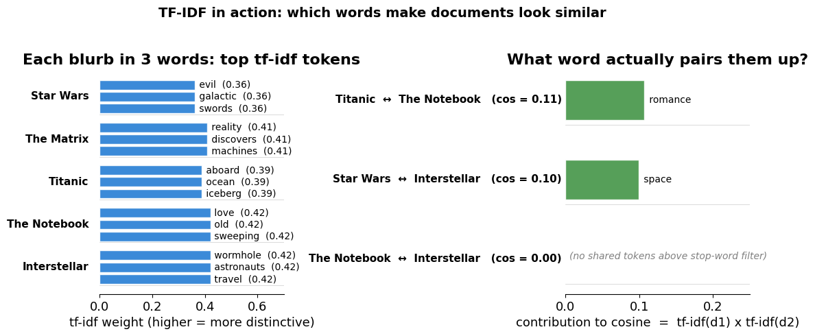
print('Romance pair drives Titanic ↔ Notebook; "space" pairs Star Wars and Interstellar. No genres needed.')
Romance pair drives Titanic ↔ Notebook; "space" pairs Star Wars and Interstellar. No genres needed.
Live Demo: TF-IDF in action — “Because you liked...”
The same trick on real MovieLens data: take a richer item vector (genres + tags + decade + popularity, all weighted with TF-IDF) and use cosine similarity to find the nearest — and furthest — neighbours.
Source
import warnings
# Richer item vector: combine FOUR feature sources, all TF-IDF + L2-normalised,
# then concatenated with per-source weights that SUM TO 1.00:
#   genres (rare combos weighted), user tags (theme/style),
#   release decade (era), popularity bucket (blockbuster vs niche).
from sklearn.feature_extraction.text import TfidfVectorizer
from sklearn.preprocessing import normalize
import scipy.sparse as sp

tags_df = pd.read_csv('ml-latest-small/tags.csv')
tag_text = (tags_df.groupby('movieId')['tag']
            .apply(lambda s: ' '.join(s.astype(str).str.lower())))

Xg = TfidfVectorizer(token_pattern=r'[^ ]+').fit_transform(
    movies['genres'].str.replace('|', ' ', regex=False).str.lower())
Xt = TfidfVectorizer(stop_words='english', min_df=2, max_features=2000,
                     token_pattern=r'[a-z][a-z\-]+').fit_transform(
    movies['movieId'].map(tag_text).fillna(''))
year = pd.to_numeric(movies['title'].str.extract(r'\((\d{4})\)', expand=False), errors='coerce')
decade_str = (year // 10 * 10).fillna(-1).astype(int).astype(str)
Xy = TfidfVectorizer(token_pattern=r'[^ ]+').fit_transform(decade_str)
rcount = ratings.groupby('movieId').size()
pop = pd.qcut(movies['movieId'].map(rcount).fillna(0), q=4,
              duplicates='drop', labels=['lo', 'midlo', 'midhi', 'hi'])
Xp = TfidfVectorizer(token_pattern=r'[^ ]+').fit_transform(pop.astype(str))

# L2-normalise each source, concatenate with weights summing to 1.
Xg_n, Xt_n, Xy_n, Xp_n = (normalize(M) for M in (Xg, Xt, Xy, Xp))
WEIGHTS = {'Genres': 0.40, 'Tags': 0.30, 'Decade': 0.20, 'Popularity': 0.10}
assert abs(sum(WEIGHTS.values()) - 1.0) < 1e-9, 'WEIGHTS should sum to 1.00'

PARTS = [('Genres', Xg_n), ('Tags', Xt_n),
         ('Decade', Xy_n), ('Popularity', Xp_n)]
DIMS = {name: M.shape[1] for name, M in PARTS}
TOTAL_DIM = sum(DIMS.values())

feature_matrix = sp.hstack(
    [WEIGHTS[name] * M for name, M in PARTS]).tocsr()
# Per-row norms vary because some movies are missing tags or popularity buckets,
# so a piece can be the zero vector instead of unit-normalized.
ROW_NORMS = np.sqrt(np.asarray(
    feature_matrix.multiply(feature_matrix).sum(axis=1)).ravel())
sim_matrix = cosine_similarity(feature_matrix)

movies['_tags']   = movies['movieId'].map(tag_text).fillna('')
movies['_decade'] = decade_str.values
movies['_popbkt'] = pop.astype(str).values

# Bar-stack colors only -- the feature sheet itself stays monochrome.
SOURCE_COLORS = {'Genres': '#1976d2', 'Tags': '#388e3c',
                 'Decade': '#f57c00', 'Popularity': '#7b1fa2'}


def _group_contribs(i, j):
    """Cosine(i,j) split per feature group; pieces sum to cosine(i,j).

    cos(i,j) = sum_k w_k^2 * <Xk_i, Xk_j>  /  (||row_i|| * ||row_j||)
    so each piece's contribution = w_k^2 * <Xk_i, Xk_j> / (||row_i|| * ||row_j||).
    """
    denom = ROW_NORMS[i] * ROW_NORMS[j]
    if denom == 0:
        return {name: 0.0 for name, _ in PARTS}
    parts = {}
    for name, M in PARTS:
        inner = (M[i] @ M[j].T).toarray().ravel()[0]
        parts[name] = WEIGHTS[name]**2 * inner / denom
    return parts


def _wrap_words(words, max_chars=26, sep=' · '):
    """Pack words into lines of <= max_chars characters, joined by `sep`."""
    lines, line = [], ''
    for w in words:
        test = line + (sep if line else '') + w
        if len(test) > max_chars and line:
            lines.append(line); line = w
        else:
            line = test
    if line:
        lines.append(line)
    return lines


def show_similar(movie_title, n_top=5, n_bottom=3):
    """Tidy feature sheet (LEFT) + most/least similar bars (RIGHT).
    Feature sheet is monochrome with a clean type hierarchy.
    Bars stack contributions by source so students see WHY each pair matches."""
    match = movies[movies['title'].str.contains(movie_title, case=False, regex=False)]
    idx = match.index[0]
    row = movies.loc[idx]
    sims = pd.Series(sim_matrix[idx], index=movies.index)
    top = sims.sort_values(ascending=False).iloc[1:n_top + 1]
    bot = sims[sims > 0].sort_values(ascending=True).iloc[:n_bottom]

    fig = plt.figure(figsize=(12.5, 5.6))
    # wspace tight: bar y-labels live INSIDE the bars now, no gap needed.
    gs = fig.add_gridspec(2, 2, width_ratios=[0.30, 0.70],
                          height_ratios=[n_top, n_bottom + 0.6],
                          wspace=0.08, hspace=0.45)

    # ============================ LEFT: tidy feature sheet ============================
    ax_l = fig.add_subplot(gs[:, 0])
    ax_l.set_xlim(0, 1); ax_l.set_ylim(0, 1); ax_l.axis('off')
    ax_l.add_patch(mpatches.FancyBboxPatch(
        (0.0, 0.0), 1.0, 1.0, boxstyle='round,pad=0.02',
        facecolor='#fafafa', edgecolor='#cfcfcf', lw=1.0, zorder=0))

    # Big headline = the movie title (the query). One unified colour throughout.
    BODY = '#222'
    MUTED = '#888'
    y = 0.94
    ax_l.text(0.06, y, row['title'], fontsize=14, fontweight='bold', color=BODY)
    y -= 0.052
    ax_l.text(0.06, y, 'feature sheet', fontsize=9, color=MUTED, style='italic')
    y -= 0.030
    ax_l.plot([0.06, 0.94], [y, y], color='#d8d8d8', lw=0.8)
    y -= 0.035

    # Body = all keywords, one consistent small style with tiny section labels.
    genres = [g for g in row['genres'].split('|') if g != '(no genres listed)']
    tag_list = [t for t in row['_tags'].split() if t]
    top_tags = pd.Series(tag_list).value_counts().head(8).index.tolist() if tag_list else []
    decade_label = (row['_decade'] + 's') if row['_decade'].isdigit() else 'unknown'
    pop_label = {'lo': 'low', 'midlo': 'mid-low', 'midhi': 'mid-high',
                 'hi': 'high'}.get(row['_popbkt'], row['_popbkt'])

    sections = [
        ('genres',     genres if genres else ['—']),
        ('user tags',  top_tags if top_tags else ['—']),
        ('decade',     [decade_label]),
        ('popularity', [pop_label]),
    ]
    for label, vals in sections:
        ax_l.text(0.06, y, label, fontsize=8, color=MUTED,
                  fontweight='bold')
        y -= 0.033
        for ln in _wrap_words(vals):
            ax_l.text(0.09, y, ln, fontsize=9.5, color=BODY)
            y -= 0.030
        y -= 0.013

    # Caption (medium) sits IMMEDIATELY below the keyword body -- no big gap.
    y -= 0.005
    ax_l.plot([0.06, 0.94], [y, y], color='#d8d8d8', lw=0.8)
    y -= 0.030
    ax_l.text(0.06, y, 'vector pieces', fontsize=8, color=MUTED, fontweight='bold')
    pieces_str = ' + '.join(f'{DIMS[n]}' for n, _ in PARTS)
    y -= 0.030
    ax_l.text(0.06, y, f'dims     {pieces_str} = {TOTAL_DIM:,}',
              fontsize=8, color=BODY, family='monospace')
    weights_str = ' + '.join(f'{WEIGHTS[n]:.2f}' for n, _ in PARTS)
    y -= 0.030
    ax_l.text(0.06, y, f'weights  {weights_str} = 1.00',
              fontsize=8, color=BODY, family='monospace')

    # ============================ RIGHT: stacked bars =================================
    def stacked_bars(ax, indices, title, header_color, with_legend=False):
        # Short titles -- inline labels mean we need to fit ~22 chars inside the bar.
        labels = [(movies.loc[i, 'title'][:24] + '…') if len(movies.loc[i, 'title']) > 24
                  else movies.loc[i, 'title'] for i in indices]
        contribs = [_group_contribs(idx, j) for j in indices]
        ypos = np.arange(len(indices))
        left = np.zeros(len(indices))
        for name, _ in PARTS:
            vals = np.array([c[name] for c in contribs])
            ax.barh(ypos, vals, left=left, color=SOURCE_COLORS[name],
                    edgecolor='white', label=name if with_legend else None)
            left += vals
        # Inline movie labels: place INSIDE the bar when it's wide enough,
        # otherwise OUTSIDE to the right so a 0.03 bar doesn't get covered.
        for j, (lbl, total) in enumerate(zip(labels, left)):
            if total >= 0.20:
                ax.text(0.015, j, lbl, va='center', fontsize=10, color='#222', ha='left',
                        bbox=dict(facecolor='white', alpha=0.85, edgecolor='none',
                                  boxstyle='round,pad=0.18'))
                ax.text(total + 0.012, j, f'{total:.2f}',
                        va='center', fontsize=10, color='#222')
            else:
                ax.text(total + 0.012, j, f'{total:.2f}  {lbl}',
                        va='center', fontsize=10, color='#222')
        ax.set_yticks([])
        ax.invert_yaxis()
        ax.set_xlim(0, max(1.05, left.max() * 1.18))
        ax.set_title(title, fontweight='bold', color=header_color, loc='left', pad=6)
        ax.spines[['top', 'right', 'left']].set_visible(False)
        ax.tick_params(axis='y', left=False)

    ax_t = fig.add_subplot(gs[0, 1])
    stacked_bars(ax_t, list(top.index), 'Most similar  (cosine, stacked by source)',
                 '#2e7d32', with_legend=True)
    ax_t.tick_params(axis='x', labelbottom=False)
    ax_t.legend(loc='lower right', fontsize=9, frameon=False, ncol=4,
                bbox_to_anchor=(1.0, 1.04))

    ax_b = fig.add_subplot(gs[1, 1], sharex=ax_t)
    stacked_bars(ax_b, list(bot.index), 'Least similar', '#c62828')
    ax_b.set_xlabel('Cosine similarity  (= Σ contributions across feature groups)')

    fig.suptitle(f'Because you liked: {row["title"]}', fontweight='bold',
                 fontsize=14, y=0.995)
    # ax_l uses axis('off'), which tight_layout flags as 'incompatible' --
    # but the manual rect gives the layout we want, so suppress the noise.
    with warnings.catch_warnings():
        warnings.simplefilter('ignore', UserWarning)
        plt.tight_layout(rect=[0, 0, 1, 0.965])
    plt.show()


show_similar('Toy Story (1995)')
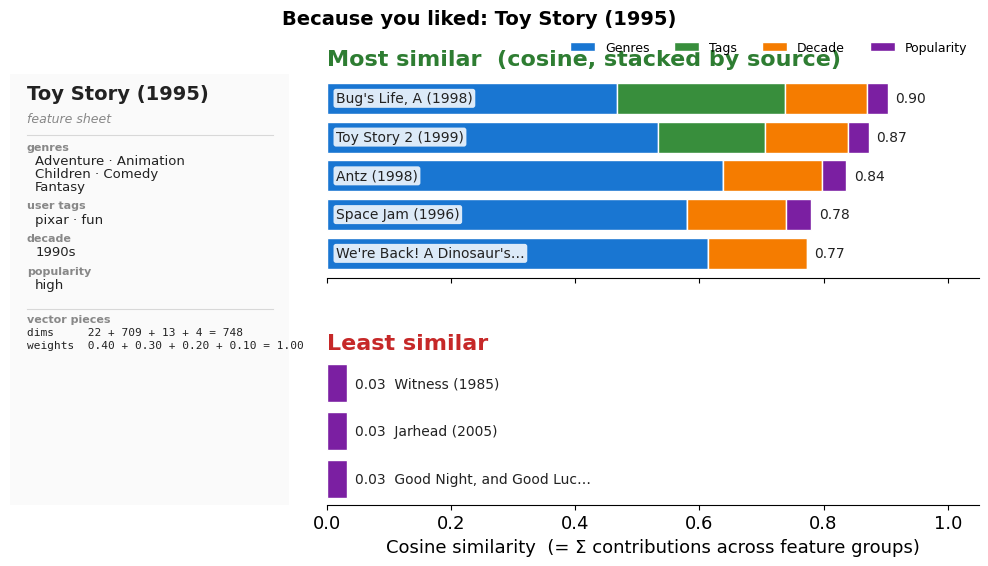
…and for Forrest Gump
Source
show_similar('Forrest Gump')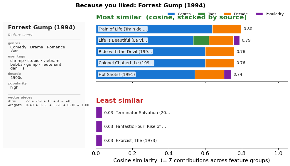
Where TF-IDF still falls short
TF-IDF only sees the exact words you wrote. It misses everything else:
| Problem | Example |
|---|---|
| Synonyms | “automobile” and “car” treated as unrelated columns |
| Polysemy | “bank” (river) vs “bank” (money) collapsed into one weight |
| Theme vs. words | A comedy and a horror both about “space” get a high score |
| Order & syntax | “dog bites man” and “man bites dog” produce identical vectors |
The fix: learn a dense embedding where direction = meaning (Word2Vec, BERT, sentence transformers). That’s the next slide, and the topic of Session 9.
Word Embeddings: meaning becomes direction
TF-IDF still treats king and queen as unrelated columns. Word embeddings (Word2Vec, GloVe) learn a dense vector per word from huge text corpora, so that directions carry meaning.
The famous example:
The “male → female” step becomes a consistent direction anywhere in the space.
Source
# Illustrative hand-placed embeddings (real Word2Vec/GloVe vectors do this in ~300-D).
words = {'man': (0.20, 0.20), 'woman': (0.20, 0.70),
         'king': (0.75, 0.30), 'queen': (0.75, 0.80)}

fig, ax = plt.subplots(figsize=(7.5, 5.5))
for w, (x, y) in words.items():
    ax.scatter(x, y, s=220, color='#1976d2', zorder=5, edgecolors='white', linewidth=2)
    ax.text(x, y + 0.04, w, fontsize=15, fontweight='bold', ha='center')

# the two parallel "male -> female" directions
for start, end in [('man', 'woman'), ('king', 'queen')]:
    ax.annotate('', xy=words[end], xytext=words[start],
                arrowprops=dict(arrowstyle='->', color='#e91e63', lw=2.5))
ax.text(0.045, 0.45, 'male → female', color='#e91e63', fontsize=11, rotation=90, va='center')
ax.text(0.595, 0.55, 'male → female', color='#e91e63', fontsize=11, rotation=90, va='center')

# king - man + woman lands on queen
pred = np.array(words['king']) - np.array(words['man']) + np.array(words['woman'])
ax.scatter(*pred, s=420, facecolors='none', edgecolors='#388e3c', linewidth=3, zorder=6)
ax.annotate('king − man + woman', xy=pred, xytext=(pred[0] - 0.40, pred[1] - 0.14),
            color='#388e3c', fontsize=12, fontweight='bold',
            arrowprops=dict(arrowstyle='->', color='#388e3c'))

ax.set_title('Analogies are parallel directions:  king − man + woman ≈ queen', fontweight='bold')
ax.set_xlim(0, 1.05)
ax.set_ylim(0, 1.0)
ax.set_aspect('equal')
ax.grid(True, alpha=0.3)
ax.spines[['top', 'right']].set_visible(False)
plt.tight_layout()
plt.show()
print('(Illustrative layout — the real vectors live in hundreds of dimensions.)')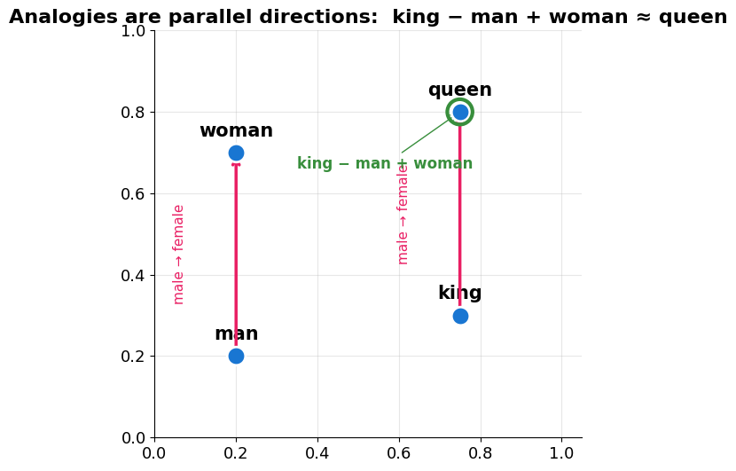
(Illustrative layout — the real vectors live in hundreds of dimensions.)
Why embeddings beat TF-IDF: similar wording, different meaning
Three short plot blurbs:
Batman — “a masked man fights crime in Gotham city at night”
Notting Hill — “a quiet man falls deeply in love with a famous actress in London”
The Punisher — “a brutal vigilante hunts down ruthless criminals across a dark metropolis”
To TF-IDF, the shared surface word “man” makes Batman look closer to a romance than to a crime drama. Embeddings know better — they read meaning, not letters.
Source
# Compare TF-IDF (counts words) with sentence embeddings (reads meaning).
# Sentence embeddings are pre-trained vectors for whole sentences; we cover them in Session 9.
import importlib.util, subprocess, sys
if importlib.util.find_spec('sentence_transformers') is None:
    subprocess.run([sys.executable, '-m', 'pip', 'install', '-q', 'sentence-transformers'], check=False)
import os, logging, warnings, contextlib
# Silence verbose model-loading output -- transformers prints a state-dict
# 'LOAD REPORT' and HF Hub prints an auth nag; neither is useful for students.
# Some of this output is written at the C level (bypassing sys.stderr),
# so we redirect file descriptor 2 in addition to setting env vars + loggers.
os.environ.setdefault('TRANSFORMERS_VERBOSITY', 'error')
os.environ.setdefault('TRANSFORMERS_NO_ADVISORY_WARNINGS', '1')
os.environ.setdefault('HF_HUB_DISABLE_PROGRESS_BARS', '1')
logging.getLogger('transformers').setLevel(logging.ERROR)
logging.getLogger('sentence_transformers').setLevel(logging.ERROR)
warnings.filterwarnings('ignore')

@contextlib.contextmanager
def _silence_fd2():
    """Suppress writes to OS file descriptor 2 (raw stderr), which Python's
    contextlib.redirect_stderr cannot catch."""
    saved = os.dup(2)
    null = os.open(os.devnull, os.O_WRONLY)
    os.dup2(null, 2)
    try:
        yield
    finally:
        os.dup2(saved, 2); os.close(saved); os.close(null)

from sentence_transformers import SentenceTransformer

blurbs = {
    'Batman':       'a masked man fights crime in Gotham city at night',
    'Notting Hill': 'a quiet man falls deeply in love with a famous actress in London',
    'The Punisher': 'a brutal vigilante hunts down ruthless criminals across a dark metropolis',
}
titles = list(blurbs)

# (1) TF-IDF cosine similarity -- the baseline.
X_tfidf = TfidfVectorizer(stop_words='english').fit_transform(blurbs.values())
sim_tfidf = cosine_similarity(X_tfidf)

# (2) Sentence-embedding cosine similarity (all-MiniLM-L6-v2, 384-D).
with _silence_fd2():
    model = SentenceTransformer('sentence-transformers/all-MiniLM-L6-v2')
emb = model.encode(list(blurbs.values()), normalize_embeddings=True)
sim_emb = emb @ emb.T

fig, axes = plt.subplots(1, 2, figsize=(10.5, 4.4))
for ax, M, title in [(axes[0], sim_tfidf, 'TF-IDF cosine similarity'),
                     (axes[1], sim_emb,   'Sentence-embedding cosine similarity')]:
    sns.heatmap(M, annot=True, fmt='.2f', cmap='RdYlGn', vmin=0, vmax=1,
                xticklabels=titles, yticklabels=titles,
                linewidths=0.5, linecolor='white', ax=ax, cbar=False,
                annot_kws={'fontsize': 13, 'fontweight': 'bold'})
    ax.set_title(title, fontweight='bold', fontsize=12)
    plt.setp(ax.get_xticklabels(), rotation=45, ha='right', fontsize=10)
    plt.setp(ax.get_yticklabels(), rotation=45, ha='right', fontsize=10)

plt.suptitle('TF-IDF gets fooled by the shared word "man"; embeddings recognise the meaning',
             fontsize=12.5, fontweight='bold', y=1.02)
plt.tight_layout()
plt.show()
print(f'TF-IDF says Batman is closer to Notting Hill ({sim_tfidf[0,1]:.2f}) than to The Punisher ({sim_tfidf[0,2]:.2f}).')
print(f'Embeddings say Batman is closer to The Punisher ({sim_emb[0,2]:.2f}) than to Notting Hill ({sim_emb[0,1]:.2f}).')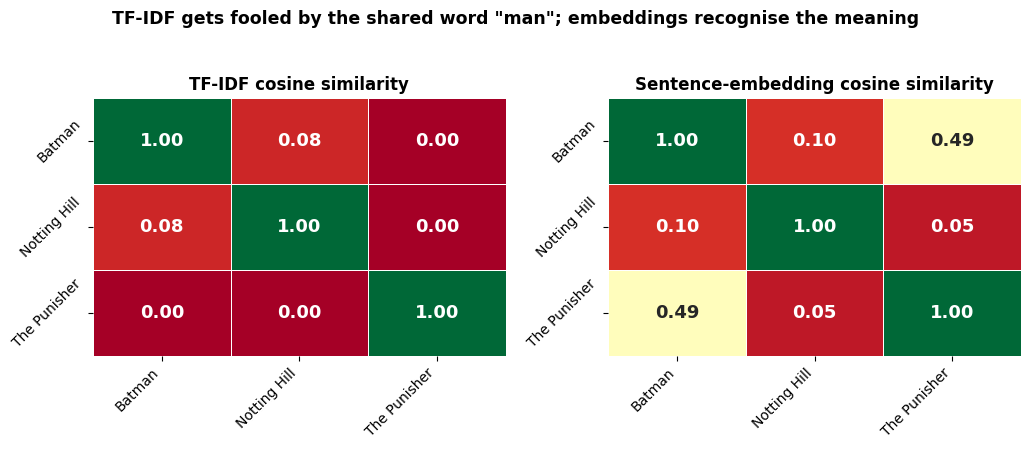
TF-IDF says Batman is closer to Notting Hill (0.08) than to The Punisher (0.00).
Embeddings say Batman is closer to The Punisher (0.49) than to Notting Hill (0.10).
The bigger picture: Information Retrieval
Information Retrieval (IR) is finding material (usually documents) of an unstructured nature that satisfies an information need from within large collections. — Manning, Raghavan & Schütze, Introduction to Information Retrieval (2008)
A recommender returning “items similar to your profile” is doing exactly this — it is a search engine whose query is you.
That reframing lets us borrow IR’s evaluation toolkit: how good is a ranked list of results?
Evaluating a ranked list: Precision & Recall
Label each returned item relevant or not, then compare to the truth:
| relevant | not relevant | |
|---|---|---|
| retrieved | TP — True Positive | FP — False Positive |
| not retrieved | FN — False Negative | TN — True Negative |
Precision — of what I returned, how much was good?
Recall — of all good items, how many did I find?
F₁ — their harmonic mean, handy when balancing both.
Return more items → recall rises, precision usually falls. Report metrics k (the top-k items).
Source
# Worked example: 100 ranked items, 10 of them relevant; a decent recommender front-loads them.
rng = np.random.default_rng(1)
N, R = 100, 10
ranked = np.zeros(N, dtype=int)
ranked[np.sort(rng.choice(np.arange(0, 40), size=R, replace=False))] = 1   # relevants front-loaded

k = np.arange(1, N + 1)
tp = np.cumsum(ranked)
precision = tp / k
recall    = tp / R
f1 = np.divide(2 * precision * recall, precision + recall,
               out=np.zeros_like(precision), where=(precision + recall) > 0)


def smooth(y, w=7):
    pad = w // 2
    padded = np.pad(y, pad, mode='edge')
    return np.convolve(padded, np.ones(w) / w, mode='valid')


f1_smooth = smooth(f1)
# Find the two visible local maxima of F1@k with scipy.signal.find_peaks.
# Sort the detected peaks by k; the first is the high-precision-low-recall peak,
# the last is the balanced-trade-off peak (also where recall has saturated).
from scipy.signal import find_peaks
peaks, _ = find_peaks(f1_smooth, distance=5, prominence=0.01)
if len(peaks) >= 2:
    early_peak, late_peak = int(peaks[0]), int(peaks[-1])
else:
    # fallback: split on the global max
    g = int(np.argmax(f1_smooth))
    early_peak = int(np.argmax(f1_smooth[:max(g, 1)]))
    late_peak  = g
k_early, k_late = early_peak + 1, late_peak + 1

fig, (ax1, ax2) = plt.subplots(1, 2, figsize=(11, 4.3))

# (1) Precision & recall as k grows.
ax1.plot(k, precision, color='#1976d2', lw=1.2, alpha=0.35)
ax1.plot(k, recall,    color='#388e3c', lw=1.2, alpha=0.35)
ax1.plot(k, smooth(precision), color='#1976d2', lw=2.6, label='Precision@k')
ax1.plot(k, smooth(recall),    color='#388e3c', lw=2.6, label='Recall@k')
for kk in (1, 5, 10):
    ax1.axvline(kk, color='gray', ls='--', alpha=0.4)
ax1.set_xlabel('k = size of the recommended list')
ax1.set_ylabel('score')
ax1.set_title('Precision falls, recall rises', fontweight='bold')
ax1.legend(loc='center right')
ax1.spines[['top', 'right']].set_visible(False)

# (2) F1@k with both sweet spots annotated.
ax2.plot(k, f1, color='#7b1fa2', lw=1.2, alpha=0.35)
ax2.plot(k, f1_smooth, color='#7b1fa2', lw=2.6, label='F1@k')
ax2.axvline(k_early, color='#1976d2', ls='--', lw=1.4)
ax2.axvline(k_late,  color='#d32f2f', ls='--', lw=1.4)
ax2.set_ylim(0, 0.55)   # leave headroom for the title and the annotations.
ax2.annotate(f'k={k_early}: precision-heavy\nP={precision[k_early-1]:.2f}  R={recall[k_early-1]:.2f}',
             xy=(k_early, f1_smooth[early_peak]),
             xytext=(k_early - 14, 0.18),
             fontsize=9, color='#1976d2', ha='left',
             arrowprops=dict(arrowstyle='->', color='#1976d2', lw=1))
ax2.annotate(f'k={k_late}: recall-heavy\nP={precision[k_late-1]:.2f}  R={recall[k_late-1]:.2f}',
             xy=(k_late, f1_smooth[late_peak]),
             xytext=(k_late + 8, 0.20),
             fontsize=9, color='#d32f2f', ha='left',
             arrowprops=dict(arrowstyle='->', color='#d32f2f', lw=1))
ax2.set_xlabel('k')
ax2.set_ylabel('F1 score')
ax2.set_title('F1@k has two sweet spots', fontweight='bold')
ax2.legend(loc='upper right')
ax2.spines[['top', 'right']].set_visible(False)

plt.tight_layout()
plt.show()
print(f'Two sweet spots: k={k_early} (precision-heavy) and k={k_late} (balanced trade-off).')
print(f'At k=10:  P={precision[9]:.2f}, R={recall[9]:.2f}, F1={f1[9]:.2f}.')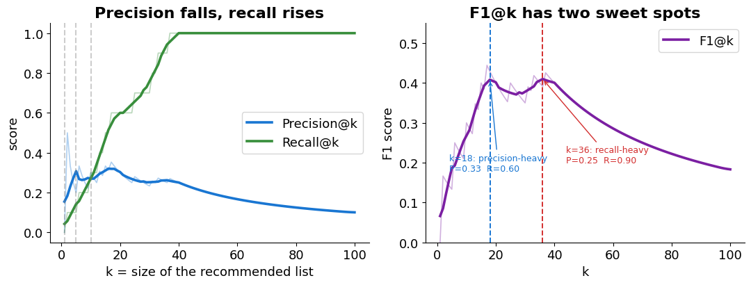
Two sweet spots: k=18 (precision-heavy) and k=36 (balanced trade-off).
At k=10:  P=0.30, R=0.30, F1=0.30.
Limitations of Content-Based Methods
Even after stacking richer signals — genres + tags + decade + popularity in our demo — three structural problems remain:
Feature-engineering bottleneck — every column is a signal someone had to design, label, and maintain. Tags need curators; cast lists need a source like IMDB; missing fields (no tags, no popularity bucket) silently weaken the vector. And TF-IDF still can’t tell car from automobile, no matter how many columns we add.
No serendipity — you only ever get more of the same. Aggarwal calls this over-specialization: even when a great pick lies in an unfamiliar category (your first Ethiopian restaurant), the recommender keeps proposing variations of what you already know.
Curse of dimensionality — richer features mean huge, sparse vectors where distance metrics blur (cf. the earlier slide on ).
Next lecture: matrix factorization. Drop the hand-designed columns and let the data discover which dimensions matter — including the implicit ones (mood, pacing, “feels like a 90s indie”) that no tag captures.
Cold Start: Partially Solved
Content-based methods can handle new items — as long as they have features (genres, description, image), we can build a vector and compare.
But new users remain a problem: without any ratings, we have no profile vector to match against.
Remember this — we’ll revisit cold start in every remaining lecture.
Key Takeaways
Everything becomes a vector — items, users, text, images — in one shared feature space.
Similarity is geometry: cosine = angle (ignores length), Euclidean = distance, dot product = both.
Content-based recommending = match a user-profile vector to item vectors (“because you liked…”).
TF-IDF & embeddings turn unstructured data into vectors automatically — the same similarity tools apply.
Evaluate a ranked list with Precision@k / Recall@k — it’s Information Retrieval.
Cold start: fine for new items, fails for new users; plus no serendipity and hand-crafted features don’t scale.
**→ Next lecture: Matrix Factorization — let the data discover the features.