Session 4: ML Model Training & Holistic Evaluation - Data Science Workflow & Applications

A practical tour from training to responsible deployment

Overview & Learning Goals¶

By the end of this notebook you will be able to:

Train an AutoML ensemble (AutoGluon) on a real tabular dataset
Evaluate model performance with cross-validated metrics and error bars
Calibrate the model to a target precision level; plot PR curves with uncertainty tubes
Interpret predictions via permutation feature importance
Assess calibration rigorously using ECE, MCE, and reliability diagrams
Measure energy consumption of individual base learners via CodeCarbon
Quantify robustness under tabular perturbations via tab-err
Audit fairness using demographic parity and equalized odds with Fairlearn

Workflows¶

Platform	Key Features	Best For
Google Vertex AI	AutoML, training, deployment, monitoring, and MLOps.	Cloud-based, enterprise-scale ML.
AWS SageMaker	Jupyter notebooks, training, deployment, AutoML, and MLOps.	AWS ecosystem users.
Azure Machine Learning	Drag-and-drop ML, AutoML, and MLOps.	Microsoft ecosystem users.
Databricks	Collaborative notebooks, Spark-based processing, MLflow integration.	Big data + ML workflows.
Dataiku	Low-code ML, AutoML, and collaboration.	Business analysts and data teams.
Domino Data Lab	Model development, deployment, and monitoring.	Enterprise MLOps.
H2O.ai	AutoML, scalable ML, and deployment.	Automated model building.

Workflows¶

End-to-end workflow frameworks haven’t really gained popularity
Instead most researchers/engineers use a dynamic / changing set of tools/libraries
Here, we follow that trend and teach you some of those solutions
But: no matter what, two things are imporant
- Documentation
  - Data sheets
  - Versioned code (git)
  - Model Cards
- Robust evaluations (Error Bars)

Model Cards¶

More reproducibility
Promoted by HuggingFace
Should contain
- ML Model
- Intended usage and limitations
- Training parameter / experimental conditions
- Data sets for training and evaluation
- Evaluation results

Mitchell et al. (2019)

Error Bars¶

Often we don’t know which model / HPs are optimal
Comparisons of models require error bars
With error bars, claimed new SOTA often is not really better

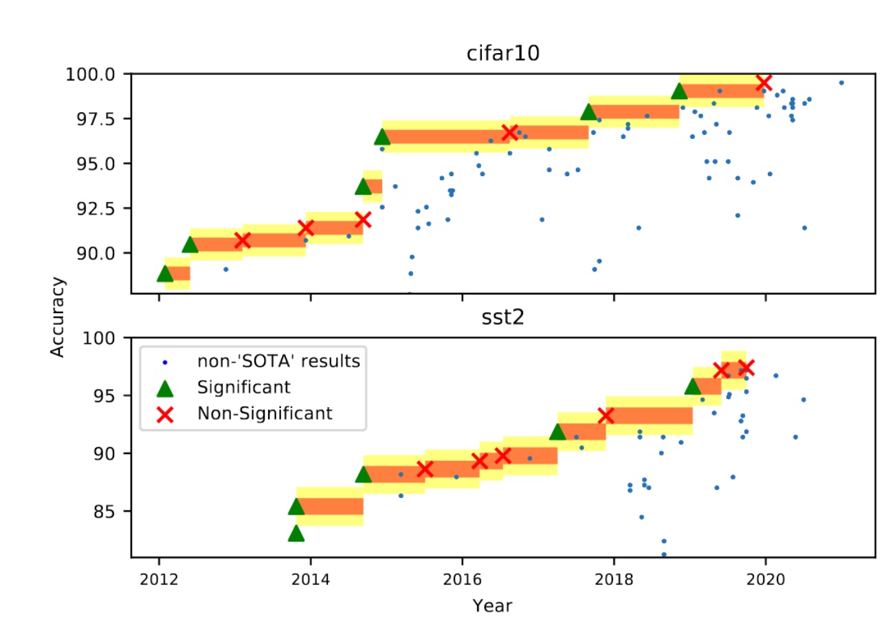
Accounting for variance in ML Benchmarks

Bouthillier et al. (2021)

How to compute Error Bars?¶

Parametric Distributions Steinbach et al. (2022)
Cross-validation (as in Bouthillier et al. (2021))

Dataset: Adult Income (OpenML ID 1590)¶

Task: Predict whether a person earns >50K USD/year (binary classification)

Why this dataset?

Real-world socioeconomic data with class imbalance (~24% positive) — calibration matters
Contains sensitive attributes (sex, race) — fairness audit is meaningful
Mix of numerical + categorical features — tests robustness to noise/missing values
~48 840 rows, 14 features — fast to train, statistically reliable CV estimates

Reference: Kohavi & Becker (1994). UCI Adult dataset. UCI ML Repository.

# ── Core imports ──────────────────────────────────────────────────────────────
import warnings, os, json
warnings.filterwarnings('ignore')

import numpy as np
import pandas as pd
import matplotlib.pyplot as plt
import matplotlib.patches as mpatches
from matplotlib.lines import Line2D

from sklearn.datasets import fetch_openml
from sklearn.model_selection import StratifiedKFold
from sklearn.metrics import (
    classification_report, precision_recall_curve,
    brier_score_loss, average_precision_score
)
from sklearn.calibration import calibration_curve

RANDOM_STATE = 42
np.random.seed(RANDOM_STATE)

import pandas as pd, numpy as np
import openml

dataset = openml.datasets.get_dataset(1590)
df, *_ = dataset.get_data(dataset_format="dataframe")

# Binarise target: 1 = '>50K', 0 = '<=50K'
df['target'] = (df['class'].str.strip().isin(['>50K', '>50K.'])).astype(int)
df = df.drop(columns=['class'])

print(df.shape, df['target'].value_counts().to_dict())
df.head(3)

(48842, 15) {0: 37155, 1: 11687}

Error Bars with Cross-Validated Model Evaluation¶

K-Fold Cross-Validation corrects this by averaging over $K$ non-overlapping folds:

\hat{\mu}_m = \frac{1}{K}\sum_{k=1}^{K} m(\mathbf{y}^{(k)},\hat{\mathbf{y}}^{(k)}), \quad \hat{\sigma}_m = \sqrt{\frac{1}{K-1}\sum_{k=1}^{K}\left(m_k - \hat{\mu}_m\right)^2}

(1)

where $m$ is any scalar metric (accuracy, F1, …) and superscripts index the held-out fold.

Kohavi & others (1995)

AutoGluon — AutoML Model Selection¶

AutoGluon trains multiple base learners (LightGBM, XGBoost, CatBoost, ExtraTrees, NNs, …) and stacks them via multi-layer ensembling:

\hat{p}_{\text{ens}}(x) = \sum_{j=1}^{J} w_j \, \hat{p}_j(x), \quad \sum_{j} w_j = 1, \; w_j \geq 0

(2)

Weights $w_j$ are learned by a meta-learner trained on out-of-fold predictions (avoids over-fitting).

presets='medium_quality' + time_limit=120 s → fast, reproducible
num_bag_folds=5 → internal CV for reliable OOF probabilities

Erickson et al. (2020)

# ── Stratified K-Fold CV with AutoGluon ───────────────────────────────────────
from autogluon.tabular import TabularPredictor
from sklearn.model_selection import StratifiedKFold
from sklearn.metrics import classification_report
import shutil, os

X = df.drop(columns=['target'])
y = df['target']

skf = StratifiedKFold(n_splits=5, shuffle=True, random_state=42)
fold_reports, fold_probas, fold_tests = [], [], []

for fold_idx, (train_idx, test_idx) in enumerate(skf.split(X, y)):
    X_tr, X_te = X.iloc[train_idx], X.iloc[test_idx]
    y_tr, y_te = y.iloc[train_idx], y.iloc[test_idx]

    train_df = X_tr.copy(); train_df['target'] = y_tr.values

    path = f'./ag_fold_{fold_idx}'
    pred = TabularPredictor(label='target', path=path, verbosity=0)
    pred.fit(
        train_data=train_df,
        presets='medium_quality',
        time_limit=20,  # for debugging this is 1 - was 120
        num_bag_folds=0,      # outer CV already provides honest eval
        num_stack_levels=0
    )

    y_pred  = pred.predict(X_te)
    y_proba = pred.predict_proba(X_te)[1].values

    report = classification_report(y_te, y_pred, output_dict=True)
    fold_reports.append(report)
    fold_probas.append(y_proba)
    fold_tests.append((y_te.values, X_te))

    shutil.rmtree(path, ignore_errors=True)

print('CV done — 5 folds')

CV done — 5 folds

# ── Aggregate metrics across folds ────────────────────────────────────────────
metrics_to_plot = ['precision', 'recall', 'f1-score']
classes         = ['0', '1']
also_accuracy   = True

results = {}   # results[class][metric] = list of fold values
for cls in classes:
    results[cls] = {m: [] for m in metrics_to_plot}
results['accuracy'] = []

for r in fold_reports:
    for cls in classes:
        for m in metrics_to_plot:
            results[cls][m].append(r[cls][m])
    results['accuracy'].append(r['accuracy'])

# Convert to arrays
for cls in classes:
    for m in metrics_to_plot:
        results[cls][m] = np.array(results[cls][m])

def _plot_cv():
    fig, axes = plt.subplots(1, 2, figsize=(11, 4), sharey=True)
    colors = ['#4C72B0', '#DD8452', '#55A868']
    
    for ax, cls in zip(axes, ['0', '1']):
        for i, m in enumerate(metrics_to_plot):
            vals = results[cls][m]
            ax.bar(i, vals.mean(), yerr=vals.std(), color=colors[i],
                   capsize=6, alpha=0.85, label=m)
        ax.set_xticks(range(3)); ax.set_xticklabels(metrics_to_plot, rotation=15)
        ax.set_ylim(0, 1.05); ax.set_title(f'Class {cls} — mean ± 1 std (5-fold)')
        ax.set_ylabel('Score')
    
    acc_vals = np.array(results['accuracy'])
    fig.suptitle(f'CV Metrics  |  Accuracy: {acc_vals.mean():.3f} ± {acc_vals.std():.3f}',
                 fontsize=13)
    plt.tight_layout(); plt.show()

_plot_cv()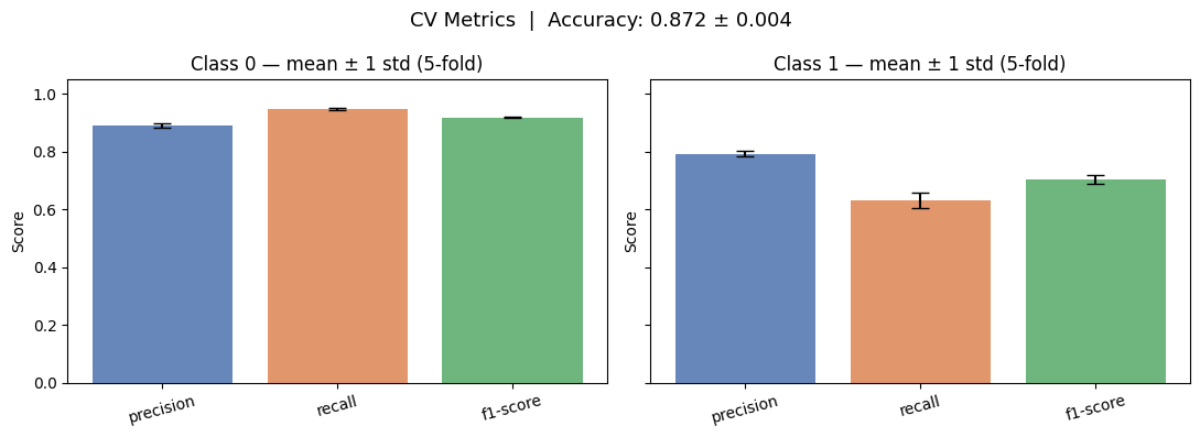

Precision-Recall & Threshold Calibration¶

Motivation¶

With class imbalance (≈24% positive), accuracy is misleading. We want to control the Precision-Recall trade-off.

For a decision threshold $\tau \in [0,1]$ :

\text{Precision}(\tau) = \frac{\text{TP}(\tau)}{\text{TP}(\tau)+\text{FP}(\tau)}, \quad \text{Recall}(\tau) = \frac{\text{TP}(\tau)}{\text{TP}(\tau)+\text{FN}(\tau)}

(3)

The area under the PR curve (AUPRC) summarises performance across all thresholds:

\text{AUPRC} = \int_0^1 P(R)\, dR \approx \sum_k P_k (R_k - R_{k-1})

(4)

Davis & Goadrich (2006)

# ── Compute PR curves per fold, interpolate to common recall grid ──────────────
from sklearn.metrics import precision_recall_curve, average_precision_score

recall_grid = np.linspace(0, 1, 200)
pr_interp_list = []
auprc_list     = []

for (y_te_vals, _), y_pr in zip(fold_tests, fold_probas):
    prec, rec, _ = precision_recall_curve(y_te_vals, y_pr)
    # sklearn returns descending recall; flip for interpolation
    prec_interp  = np.interp(recall_grid, rec[::-1], prec[::-1])
    pr_interp_list.append(prec_interp)
    auprc_list.append(average_precision_score(y_te_vals, y_pr))

pr_matrix  = np.vstack(pr_interp_list)   # shape (5, 200)
pr_mean    = pr_matrix.mean(axis=0)
pr_std     = pr_matrix.std(axis=0)
auprc_mean = np.mean(auprc_list)
auprc_std  = np.std(auprc_list)

def _plot_pr():
    fig, ax = plt.subplots(figsize=(8, 4.5))
    ax.plot(recall_grid, pr_mean, color='#2196F3', lw=2,label=f'Mean PR  (AUPRC={auprc_mean:.3f}±{auprc_std:.3f})')
    ax.fill_between(recall_grid, pr_mean - pr_std, pr_mean + pr_std,alpha=0.25, color='#2196F3', label='±1 std across folds')
    # Mark target precision = 0.80
    target_p = 0.80
    idx_target = np.argmax(pr_mean >= target_p)          # first index where mean >= target
    ax.axhline(target_p, ls='--', color='tomato', label=f'Target precision={target_p}')
    ax.axvline(recall_grid[idx_target], ls=':', color='tomato')
    ax.set_xlabel('Recall'); ax.set_ylabel('Precision')
    ax.set_title('Precision-Recall Curve (5-fold CV ± 1 std)')
    ax.legend(loc='lower left'); ax.set_xlim(0,1); ax.set_ylim(0,1.05)
    plt.tight_layout(); plt.show()

_plot_pr()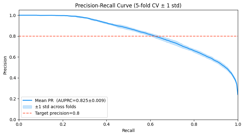

Choosing a Decision Threshold for Target Precision¶

To guarantee a minimum precision $p^*$ on unseen data:

From the mean PR curve find the smallest threshold $\hat{\tau}$ such that
$\text{Precision}(\hat{\tau}) \geq p^*$
(5)
Report the corresponding recall — this is the cost of the constraint.
Use the lower bound of the precision error tube ( $\mu - \sigma$ ) for a conservative estimate.

Practical note: Always re-tune $\hat{\tau}$ on a held-out validation set in production.

Lipton et al. (2014)

# For illustration use fold 0 probabilities + actual thresholds from sklearn
y_te0, _ = fold_tests[0]
prec_arr, rec_arr, thresh_arr = precision_recall_curve(y_te0, fold_probas[0])

target_precision = 0.80
# Find index where precision >= target (prec_arr is descending by threshold)
valid = np.where(prec_arr[:-1] >= target_precision)[0]
if len(valid) > 0:
    best_idx = valid[-1]   # highest recall that still meets precision target
    best_tau = thresh_arr[best_idx]
    best_rec = rec_arr[best_idx]
    print(f'Target precision  : {target_precision:.2f}')
    print(f'Optimal threshold : tau = {best_tau:.4f}')
    print(f'Achieved recall   : {best_rec:.4f}')
else:
    print('Target precision cannot be reached with this model.')

Target precision  : 0.80
Optimal threshold : tau = 0.9029
Achieved recall   : 0.0004

Feature Importance Analysis / XAI¶

**eXplainable AI aims at making model (decisions) more transparent
XAI is a huge field with its own conferences
It’s difficult to define metrics for XAI methods
There is no ground truth for XAI experiments (except for synthetic data sets)

Permutation Importance¶

A simple and well established XAI method.
Permutation Importance (Breiman 2001) measures how much the model relies on feature $j$ :

I_j = \hat{\mu}_m - \frac{1}{T}\sum_{t=1}^{T} m(\mathbf{y},\hat{f}(X_{\pi_t(j)}))

(6)

where $\pi_t(j)$ is the $t$ -th random permutation of column $j$ .

$I_j > 0$ : model relied on feature $j$ (shuffling hurts)
$I_j \approx 0$ : feature is uninformative or redundant

AutoGluon wraps this natively; we also compute CV error bars by averaging over folds.

Reference: Breiman (2001). Random Forests. Machine Learning, 45(1).

# ── Re-train one AutoGluon model on full training set for feature importance ───
from autogluon.tabular import TabularPredictor
from sklearn.model_selection import train_test_split

train_df_full, test_df_full = train_test_split(
    df, test_size=0.20, stratify=df['target'], random_state=42
)

pred_main = TabularPredictor(label='target', path='./ag_main', verbosity=0)
pred_main.fit(
    train_data=train_df_full,
    presets='medium_quality',
    time_limit=120,
    num_bag_folds=5,
    num_stack_levels=0
)

X_test_main  = test_df_full.drop(columns=['target'])
y_test_main  = test_df_full['target']
y_proba_main = pred_main.predict_proba(X_test_main)[1].values

fi_df = pred_main.feature_importance(
    data=test_df_full, num_shuffle_sets=5, subsample_size=5000
)

def _plot_feat_imp():
    top_n = 10
    fi_top = fi_df.head(top_n).sort_values('importance', ascending=True)
    fig, ax = plt.subplots(figsize=(8, 5))
    ax.barh(fi_top.index, fi_top['importance'],
            xerr=fi_top['stddev'], color='#4C72B0',
            capsize=4, alpha=0.85)
    ax.set_xlabel('Permutation Importance (accuracy drop)')
    ax.set_title(f'Top {top_n} Feature Importances (mean ± std, {5} shuffle sets)')
    plt.tight_layout(); plt.show()

print(fi_df.head(5))

               importance    stddev       p_value  n  p99_high   p99_low
capital-gain      0.05384  0.002559  6.104800e-07  5  0.059109  0.048571
occupation        0.01980  0.004602  3.263764e-04  5  0.029276  0.010324
education-num     0.01676  0.002343  4.463587e-05  5  0.021584  0.011936
age               0.01616  0.004246  5.228259e-04  5  0.024902  0.007418
relationship      0.01532  0.002305  5.965803e-05  5  0.020066  0.010574

_plot_feat_imp()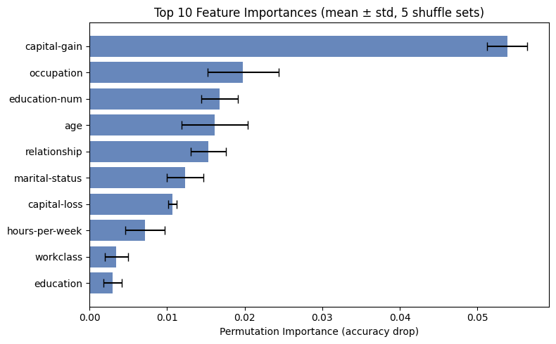

Feature Importance — Key Takeaways¶

Typical findings on the Adult dataset:

capital_gain and age are the strongest predictors — high income correlates with investment returns and seniority
education_num and hours_per_week carry significant signal
race and sex have non-zero importance → signals potential for disparate treatment (see Fairness section)

Caveats

Permutation importance overestimates importance of correlated features
Correlations of variables can distort feature importance measures

Calibration of ML Predictions¶

Are important when you deploy a model in real-world applications
Can be based on a variety of metrics

Metric	Range	Pros	Cons	Use Case
Brier Score	[0, 1]	Simple, accounts for sharpness	Sensitive to class imbalance	General-purpose evaluation
Calibration Curve	Visual	Intuitive, identifies local miscalibration	Binning-dependent, not scalar	Diagnostic tool
ECE	[0, 0.5]	Scalar, interpretable	Binning-dependent	Model selection

Guo et al. (2017)

Expected Calibration Error (ECE)¶

Partition predictions into $M$ equal-width bins $B_1,\ldots,B_M$ :

\text{ECE} = \sum_{m=1}^{M} \frac{|B_m|}{N}\,\bigl|\overline{y}(B_m) - \bar{\hat{p}}(B_m)\bigr|

(7)

where $\overline{y}(B_m)$ is the empirical positive rate and $\bar{\hat{p}}(B_m)$ the mean predicted probability in bin $m$ .

Guo et al. (2017)

# ── Calibration metrics on the main test split ────────────────────────────────
from sklearn.calibration import calibration_curve, CalibratedClassifierCV
from sklearn.metrics import brier_score_loss

n_bins = 10
y_true_arr  = y_test_main.values
y_proba_arr = y_proba_main

# Raw model
frac_pos, mean_pred = calibration_curve(y_true_arr, y_proba_arr, n_bins=n_bins)
brier_raw           = brier_score_loss(y_true_arr, y_proba_arr)

# ECE / MCE (manual)
bin_edges  = np.linspace(0, 1, n_bins + 1)
ece, mce   = 0.0, 0.0
N          = len(y_true_arr)
for lo, hi in zip(bin_edges[:-1], bin_edges[1:]):
    mask  = (y_proba_arr >= lo) & (y_proba_arr < hi)
    if mask.sum() == 0: continue
    acc_b = y_true_arr[mask].mean()
    con_b = y_proba_arr[mask].mean()
    diff  = abs(acc_b - con_b)
    ece  += (mask.sum() / N) * diff
    mce   = max(mce, diff)

def _plot_calibration():
    fig, ax = plt.subplots(figsize=(6, 5))
    
    ax.plot([0,1],[0,1], ls='--', color='grey', label='Perfect calibration')
    ax.plot(mean_pred, frac_pos, marker='s', color='#2196F3', lw=2,
            label=f'AutoGluon (ECE={ece:.3f}, MCE={mce:.3f})')
    
    ax.set_xlabel('Mean Predicted Probability')
    ax.set_ylabel('Fraction of Positives')
    ax.set_title('Reliability Diagram')
    ax.legend(); ax.set_xlim(0,1); ax.set_ylim(0,1)
    plt.tight_layout(); plt.show()
    print(f'Brier Score: {brier_raw:.4f}')
    
print(f'Brier Score: {brier_raw:.4f}  |  ECE: {ece:.4f}  |  MCE: {mce:.4f}')

Brier Score: 0.0867  |  ECE: 0.0095  |  MCE: 0.0412

_plot_calibration()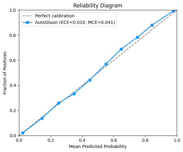

Brier Score: 0.0867

Energy Efficiency¶

Training and serving ML models has a real carbon footprint:

“Training GPT-3 emitted ~552 t CO₂eq — equivalent to ~120 US cars for a year.” — Lottick et al. (2019)

Even for tabular models, knowing the energy-accuracy trade-off guides sustainable model selection.

CodeCarbon monitors hardware power usage and converts to CO₂ equivalent:

E_{\text{CO}_2} = P_{\text{hardware}} \times t_{\text{train}} \times \text{CI}_{\text{grid}}

(8)

where $\text{CI}_{\text{grid}}$ is the carbon intensity of the electricity grid (kg CO₂/kWh).

Lottick et al. (2019)

# ── Per-model energy tracking using CodeCarbon ────────────────────────────────
# We re-train each base learner individually to measure its footprint.

from codecarbon import EmissionsTracker
from autogluon.tabular import TabularPredictor
import shutil

# Define models to compare
base_models = {
    'LightGBM': {'hyperparameters': {'GBM': {}}},
    'XGBoost':  {'hyperparameters': {'XGB': {}}},
    'ExtraTrees': {'hyperparameters': {'XT': {}}},
    'RandomForest': {'hyperparameters': {'RF': {}}},
}

energy_results = {}
for name, fit_kwargs in base_models.items():
    path = f'./ag_energy_{name}'
    tracker = EmissionsTracker(project_name=name, save_to_file=False)
    tracker.start()
    pred_e = TabularPredictor(label='target', path=path, verbosity=0)
    pred_e.fit(train_data=train_df_full, time_limit=60, **fit_kwargs)
    emissions = tracker.stop()   # kg CO2eq

    y_pred_e = pred_e.predict(X_test_main)
    acc_e    = (y_pred_e.values == y_test_main.values).mean()
    energy_results[name] = {'co2_kg': emissions, 'accuracy': acc_e}
    shutil.rmtree(path, ignore_errors=True)

def _plot_energy():
    energy_df = pd.DataFrame(energy_results).T

    fig, ax = plt.subplots(figsize=(8, 4.5))
    scatter = ax.scatter(
        energy_df['co2_kg'] * 1e6,  # convert to micro-grams for readability
        energy_df['accuracy'],
        s=120, c=range(len(energy_df)), cmap='tab10', zorder=3
    )
    for name, row in energy_df.iterrows():
        ax.annotate(name, (row['co2_kg']*1e6, row['accuracy']),
                    textcoords='offset points', xytext=(6,4), fontsize=9)
    
    ax.set_xlabel('CO2 Emissions (ug CO2eq)')
    ax.set_ylabel('Test Accuracy')
    ax.set_title('Energy vs. Accuracy Trade-off per Base Learner')
    plt.tight_layout(); plt.show()
print(pd.DataFrame(energy_results).T)

[codecarbon WARNING @ 12:01:46] Multiple instances of codecarbon are allowed to run at the same time.
[codecarbon WARNING @ 12:01:46] Error while trying to count physical CPUs: [Errno 2] No such file or directory: 'lscpu'. Defaulting to 1.
[codecarbon INFO @ 12:01:46] [setup] RAM Tracking...
[codecarbon INFO @ 12:01:46] [setup] CPU Tracking...
[codecarbon WARNING @ 12:01:46] We saw that you have a Apple M2 but we don't know it. Please contact us.
[codecarbon WARNING @ 12:01:46] No CPU tracking mode found. Falling back on estimation based on TDP for CPU. 
 Mac OS and ARM processor detected: Please enable PowerMetrics sudo to measure CPU

[codecarbon INFO @ 12:01:46] CPU Model on constant consumption mode: Apple M2
[codecarbon WARNING @ 12:01:46] No CPU tracking mode found. Falling back on CPU constant mode.
[codecarbon INFO @ 12:01:46] [setup] GPU Tracking...
[codecarbon INFO @ 12:01:46] No GPU found.
[codecarbon INFO @ 12:01:46] The below tracking methods have been set up:
                RAM Tracking Method: RAM power estimation model
                CPU Tracking Method: global constant
                GPU Tracking Method: Unspecified
            
[codecarbon INFO @ 12:01:46] >>> Tracker's metadata:
[codecarbon INFO @ 12:01:46]   Platform system: macOS-15.6.1-arm64-arm-64bit
[codecarbon INFO @ 12:01:46]   Python version: 3.12.8
[codecarbon INFO @ 12:01:46]   CodeCarbon version: 3.2.6
[codecarbon INFO @ 12:01:46]   Available RAM : 24.000 GB
[codecarbon INFO @ 12:01:46]   CPU count: 8 thread(s) in 1 physical CPU(s)
[codecarbon INFO @ 12:01:46]   CPU model: Apple M2
[codecarbon INFO @ 12:01:46]   GPU count: 0
[codecarbon INFO @ 12:01:46]   GPU model: 
[codecarbon INFO @ 12:01:52] Energy consumed for RAM : 0.000004 kWh. RAM Power : 6.0 W
[codecarbon INFO @ 12:01:52] Delta energy consumed for CPU with constant : 0.000031 kWh, power : 42.5 W
[codecarbon INFO @ 12:01:52] Energy consumed for All CPU : 0.000031 kWh
[codecarbon INFO @ 12:01:52] 0.000035 kWh of electricity and 0.000000 L of water were used since the beginning.
[codecarbon WARNING @ 12:01:52] Multiple instances of codecarbon are allowed to run at the same time.
[codecarbon WARNING @ 12:01:52] Error while trying to count physical CPUs: [Errno 2] No such file or directory: 'lscpu'. Defaulting to 1.
[codecarbon INFO @ 12:01:52] [setup] RAM Tracking...
[codecarbon INFO @ 12:01:52] [setup] CPU Tracking...
[codecarbon WARNING @ 12:01:52] We saw that you have a Apple M2 but we don't know it. Please contact us.
[codecarbon WARNING @ 12:01:52] No CPU tracking mode found. Falling back on estimation based on TDP for CPU. 
 Mac OS and ARM processor detected: Please enable PowerMetrics sudo to measure CPU

[codecarbon INFO @ 12:01:52] CPU Model on constant consumption mode: Apple M2
[codecarbon WARNING @ 12:01:52] No CPU tracking mode found. Falling back on CPU constant mode.
[codecarbon INFO @ 12:01:52] [setup] GPU Tracking...
[codecarbon INFO @ 12:01:52] No GPU found.
[codecarbon INFO @ 12:01:52] The below tracking methods have been set up:
                RAM Tracking Method: RAM power estimation model
                CPU Tracking Method: global constant
                GPU Tracking Method: Unspecified
            
[codecarbon INFO @ 12:01:52] >>> Tracker's metadata:
[codecarbon INFO @ 12:01:52]   Platform system: macOS-15.6.1-arm64-arm-64bit
[codecarbon INFO @ 12:01:52]   Python version: 3.12.8
[codecarbon INFO @ 12:01:52]   CodeCarbon version: 3.2.6
[codecarbon INFO @ 12:01:52]   Available RAM : 24.000 GB
[codecarbon INFO @ 12:01:52]   CPU count: 8 thread(s) in 1 physical CPU(s)
[codecarbon INFO @ 12:01:52]   CPU model: Apple M2
[codecarbon INFO @ 12:01:52]   GPU count: 0
[codecarbon INFO @ 12:01:52]   GPU model: 
[codecarbon INFO @ 12:01:54] Energy consumed for RAM : 0.000002 kWh. RAM Power : 6.0 W
[codecarbon INFO @ 12:01:54] Delta energy consumed for CPU with constant : 0.000017 kWh, power : 42.5 W
[codecarbon INFO @ 12:01:54] Energy consumed for All CPU : 0.000017 kWh
[codecarbon INFO @ 12:01:54] 0.000020 kWh of electricity and 0.000000 L of water were used since the beginning.
[codecarbon WARNING @ 12:01:54] Multiple instances of codecarbon are allowed to run at the same time.
[codecarbon WARNING @ 12:01:55] Error while trying to count physical CPUs: [Errno 2] No such file or directory: 'lscpu'. Defaulting to 1.
[codecarbon INFO @ 12:01:55] [setup] RAM Tracking...
[codecarbon INFO @ 12:01:55] [setup] CPU Tracking...
[codecarbon WARNING @ 12:01:55] We saw that you have a Apple M2 but we don't know it. Please contact us.
[codecarbon WARNING @ 12:01:55] No CPU tracking mode found. Falling back on estimation based on TDP for CPU. 
 Mac OS and ARM processor detected: Please enable PowerMetrics sudo to measure CPU

[codecarbon INFO @ 12:01:55] CPU Model on constant consumption mode: Apple M2
[codecarbon WARNING @ 12:01:55] No CPU tracking mode found. Falling back on CPU constant mode.
[codecarbon INFO @ 12:01:55] [setup] GPU Tracking...
[codecarbon INFO @ 12:01:55] No GPU found.
[codecarbon INFO @ 12:01:55] The below tracking methods have been set up:
                RAM Tracking Method: RAM power estimation model
                CPU Tracking Method: global constant
                GPU Tracking Method: Unspecified
            
[codecarbon INFO @ 12:01:55] >>> Tracker's metadata:
[codecarbon INFO @ 12:01:55]   Platform system: macOS-15.6.1-arm64-arm-64bit
[codecarbon INFO @ 12:01:55]   Python version: 3.12.8
[codecarbon INFO @ 12:01:55]   CodeCarbon version: 3.2.6
[codecarbon INFO @ 12:01:55]   Available RAM : 24.000 GB
[codecarbon INFO @ 12:01:55]   CPU count: 8 thread(s) in 1 physical CPU(s)
[codecarbon INFO @ 12:01:55]   CPU model: Apple M2
[codecarbon INFO @ 12:01:55]   GPU count: 0
[codecarbon INFO @ 12:01:55]   GPU model: 
[codecarbon INFO @ 12:01:57] Energy consumed for RAM : 0.000004 kWh. RAM Power : 6.0 W
[codecarbon INFO @ 12:01:57] Delta energy consumed for CPU with constant : 0.000029 kWh, power : 42.5 W
[codecarbon INFO @ 12:01:57] Energy consumed for All CPU : 0.000029 kWh
[codecarbon INFO @ 12:01:57] 0.000033 kWh of electricity and 0.000000 L of water were used since the beginning.
[codecarbon WARNING @ 12:01:57] Multiple instances of codecarbon are allowed to run at the same time.
[codecarbon WARNING @ 12:01:58] Error while trying to count physical CPUs: [Errno 2] No such file or directory: 'lscpu'. Defaulting to 1.
[codecarbon INFO @ 12:01:58] [setup] RAM Tracking...
[codecarbon INFO @ 12:01:58] [setup] CPU Tracking...
[codecarbon WARNING @ 12:01:58] We saw that you have a Apple M2 but we don't know it. Please contact us.
[codecarbon WARNING @ 12:01:58] No CPU tracking mode found. Falling back on estimation based on TDP for CPU. 
 Mac OS and ARM processor detected: Please enable PowerMetrics sudo to measure CPU

[codecarbon INFO @ 12:01:58] CPU Model on constant consumption mode: Apple M2
[codecarbon WARNING @ 12:01:58] No CPU tracking mode found. Falling back on CPU constant mode.
[codecarbon INFO @ 12:01:58] [setup] GPU Tracking...
[codecarbon INFO @ 12:01:58] No GPU found.
[codecarbon INFO @ 12:01:58] The below tracking methods have been set up:
                RAM Tracking Method: RAM power estimation model
                CPU Tracking Method: global constant
                GPU Tracking Method: Unspecified
            
[codecarbon INFO @ 12:01:58] >>> Tracker's metadata:
[codecarbon INFO @ 12:01:58]   Platform system: macOS-15.6.1-arm64-arm-64bit
[codecarbon INFO @ 12:01:58]   Python version: 3.12.8
[codecarbon INFO @ 12:01:58]   CodeCarbon version: 3.2.6
[codecarbon INFO @ 12:01:58]   Available RAM : 24.000 GB
[codecarbon INFO @ 12:01:58]   CPU count: 8 thread(s) in 1 physical CPU(s)
[codecarbon INFO @ 12:01:58]   CPU model: Apple M2
[codecarbon INFO @ 12:01:58]   GPU count: 0
[codecarbon INFO @ 12:01:58]   GPU model: 
[codecarbon INFO @ 12:02:02] Energy consumed for RAM : 0.000008 kWh. RAM Power : 6.0 W
[codecarbon INFO @ 12:02:02] Delta energy consumed for CPU with constant : 0.000055 kWh, power : 42.5 W
[codecarbon INFO @ 12:02:02] Energy consumed for All CPU : 0.000055 kWh
[codecarbon INFO @ 12:02:02] 0.000062 kWh of electricity and 0.000000 L of water were used since the beginning.

                co2_kg  accuracy
LightGBM      0.000013  0.876651
XGBoost       0.000008  0.875832
ExtraTrees    0.000013  0.853516
RandomForest  0.000024  0.860682

_plot_energy()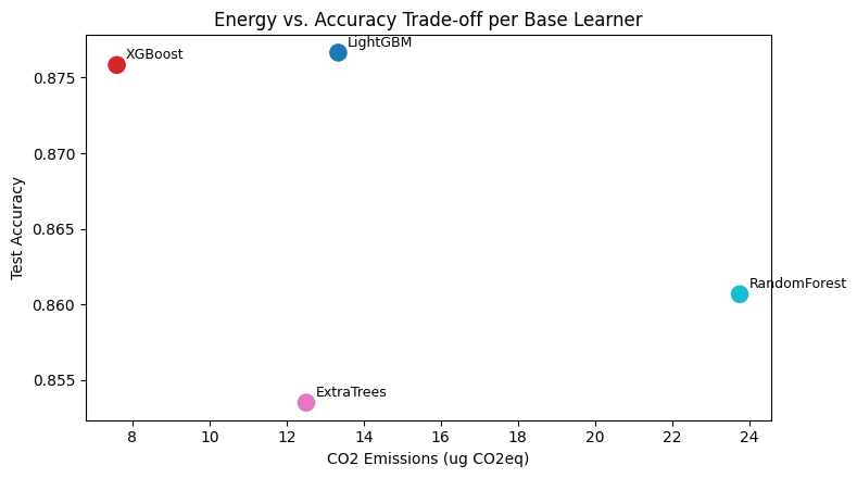

Robustness Analysis¶

tab-err Jung et al. (2025) and schelter2021jenga generates realistic errors
Helps to assess robustness of ML models

Helper function to display the perturbed results

from sklearn.datasets import load_iris

def show_result(original_df: pd.DataFrame, perturbed_df: pd.DataFrame, error_mask: pd.DataFrame | None = None) -> pd.DataFrame:
    """Simple helper function to show DataFrames after perturbing them."""
    return (
        pd.concat([original_df, perturbed_df], keys=["original", "perturbed"], axis=1)
        if error_mask is None
        else pd.concat([original_df, perturbed_df, error_mask], keys=["original", "perturbed", "error_mask"], axis=1)
    )

Train / Test Split

from sklearn.model_selection import train_test_split

X = df.drop(columns=['target'])
y = df['target']

X_train, X_test, y_train, y_test = train_test_split(
    X, y, 
    test_size=0.2, 
    random_state=42, 
    stratify=y
)

print(f"Training set size: {X_train.shape[0]}")
print(f"Testing set size: {X_test.shape[0]}")

Training set size: 39073
Testing set size: 9769

Model training¶

We train a classification model on the training data.

from sklearn.ensemble import HistGradientBoostingClassifier
from sklearn.pipeline import make_pipeline

categorical_mask = [
    False, # age
    True,  # workclass
    False, # fnlwgt
    True,  # education
    False, # education-num
    True,  # marital-status
    True,  # occupation
    True,  # relationship
    True,  # race
    True,  # sex
    False, # capital-gain
    False, # capital-loss
    False, # hours-per-week
    True   # native-country
]

clf = make_pipeline(
    HistGradientBoostingClassifier(categorical_features=categorical_mask,
    max_iter=100,
    random_state=42)
)

clf.fit(X_train, y_train)

Perturb Test Data¶

from tab_err import error_type
from tab_err.api import high_level

X_test_perturbed, error_mask = high_level.create_errors(
    data=X_test,
    error_rate=0.15,
    error_types_to_exclude=[error_type.MissingValue(), error_type.CategorySwap()]
)

show_result(X_test, X_test_perturbed, error_mask).head()

Inference on Clean and Perturbed Data¶

from sklearn.metrics import classification_report

def evaluate_model(model, X_test, y_test):
    """
    Prints a formatted report and returns basic accuracy.
    """
    y_pred = model.predict(X_test)

    # Precision, Recall, F1 per class
    report = classification_report(y_test, y_pred)
    
    print(report)

import pandas as pd
import numpy as np
from tab_err import error_type
from tab_err.api import high_level
from sklearn.metrics import precision_score, recall_score, f1_score

def calculate_manual_ece(y_true, y_proba, n_bins=10):
    bin_edges = np.linspace(0, 1, n_bins + 1)
    ece = 0.0
    N = len(y_true)
    for lo, hi in zip(bin_edges[:-1], bin_edges[1:]):
        mask = (y_proba >= lo) & (y_proba < hi)
        if mask.sum() == 0: continue
        acc_b = y_true[mask].mean()
        con_b = y_proba[mask].mean()
        ece += (mask.sum() / N) * abs(acc_b - con_b)
    return ece

def evaluate_robustness(model, X_test, y_true, error_rate=0.15, n_repeats=10):
    results = []
    y_true_values = y_true.values

    for i in range(n_repeats):
        # 1. Perturb
        X_perturbed, _ = high_level.create_errors(
            data=X_test,
            error_rate=error_rate,
            error_types_to_exclude=[error_type.MissingValue(), error_type.CategorySwap()]
        )
        
        # 2. Predict
        # Getting P(Y=1)
        y_proba = model.predict_proba(X_perturbed)
        y_proba_arr = y_proba[1].values if isinstance(y_proba, pd.DataFrame) else y_proba[:, 1]
        y_pred = (y_proba_arr >= 0.5).astype(int)
        
        # 3. Score
        metrics = {
            'repetition': i,
            'precision': precision_score(y_true_values, y_pred),
            'recall': recall_score(y_true_values, y_pred),
            'f1': f1_score(y_true_values, y_pred),
            'ece': calculate_manual_ece(y_true_values, y_proba_arr)
        }
        results.append(metrics)

    df_res = pd.DataFrame(results)
    
    return df_res

error_rates = [0.0, 0.1, 0.2, 0.3, 0.4, 0.5]
experiment_data = {rate: evaluate_robustness(clf, X_test_perturbed, y_test, rate) for rate in error_rates}

# 1. Aggregate stats across all experiments
all_stats = []
for rate, df in experiment_data.items():
    # Calculate stats for this specific error rate
    stats = df.drop(columns='repetition').agg(['mean', 'std']).T
    stats['error_rate'] = rate
    all_stats.append(stats.reset_index().rename(columns={'index': 'metric'}))

# 2. Combine and pivot for plotting
summary_df = pd.concat(all_stats)
pivot_mean = summary_df.pivot(index='error_rate', columns='metric', values='mean')
pivot_std = summary_df.pivot(index='error_rate', columns='metric', values='std')

print("--- Robustness Mean Metrics ---")
print(pivot_mean)

--- Robustness Mean Metrics ---
metric           ece        f1  precision    recall
error_rate                                         
0.0         0.009139  0.706071   0.760237  0.659110
0.1         0.012177  0.699580   0.752799  0.653464
0.2         0.019267  0.689394   0.750848  0.638580
0.3         0.024553  0.670759   0.757023  0.603293
0.4         0.026670  0.677186   0.746548  0.621514
0.5         0.036300  0.668021   0.742521  0.612746

def _plot_perturbation():
    metrics = ['precision', 'recall', 'f1', 'ece']
    fig, axes = plt.subplots(2, 2, figsize=(14, 10))
    axes = axes.flatten()
    
    for i, metric in enumerate(metrics):
        ax = axes[i]
        x = pivot_mean.index
        y = pivot_mean[metric]
        err = pivot_std[metric]
        
        # Plotting the mean line
        color = 'tab:red' if metric == 'ece' else 'tab:blue'
        ax.plot(x, y, marker='o', linestyle='-', color=color, label=f'Mean {metric}')
        
        # Shading the variance (Standard Deviation)
        ax.fill_between(x, y - err, y + err, color=color, alpha=0.15, label='±1 Std Dev')
        
        ax.set_title(f'{metric.upper()} vs. Perturbation Rate', fontsize=12, fontweight='bold')
        ax.set_xlabel('Error Rate')
        ax.set_ylabel('Score')
        ax.grid(True, which='both', linestyle='--', alpha=0.5)
        ax.legend(loc='best')
    
        # Invert ECE axis or add note: Lower is better for ECE
        if metric == 'ece':
            ax.annotate('Lower is Better', xy=(0.05, 0.9), xycoords='axes fraction', 
                        fontsize=10, color='darkred', fontweight='bold')
    
    plt.tight_layout()
    plt.show()

_plot_perturbation()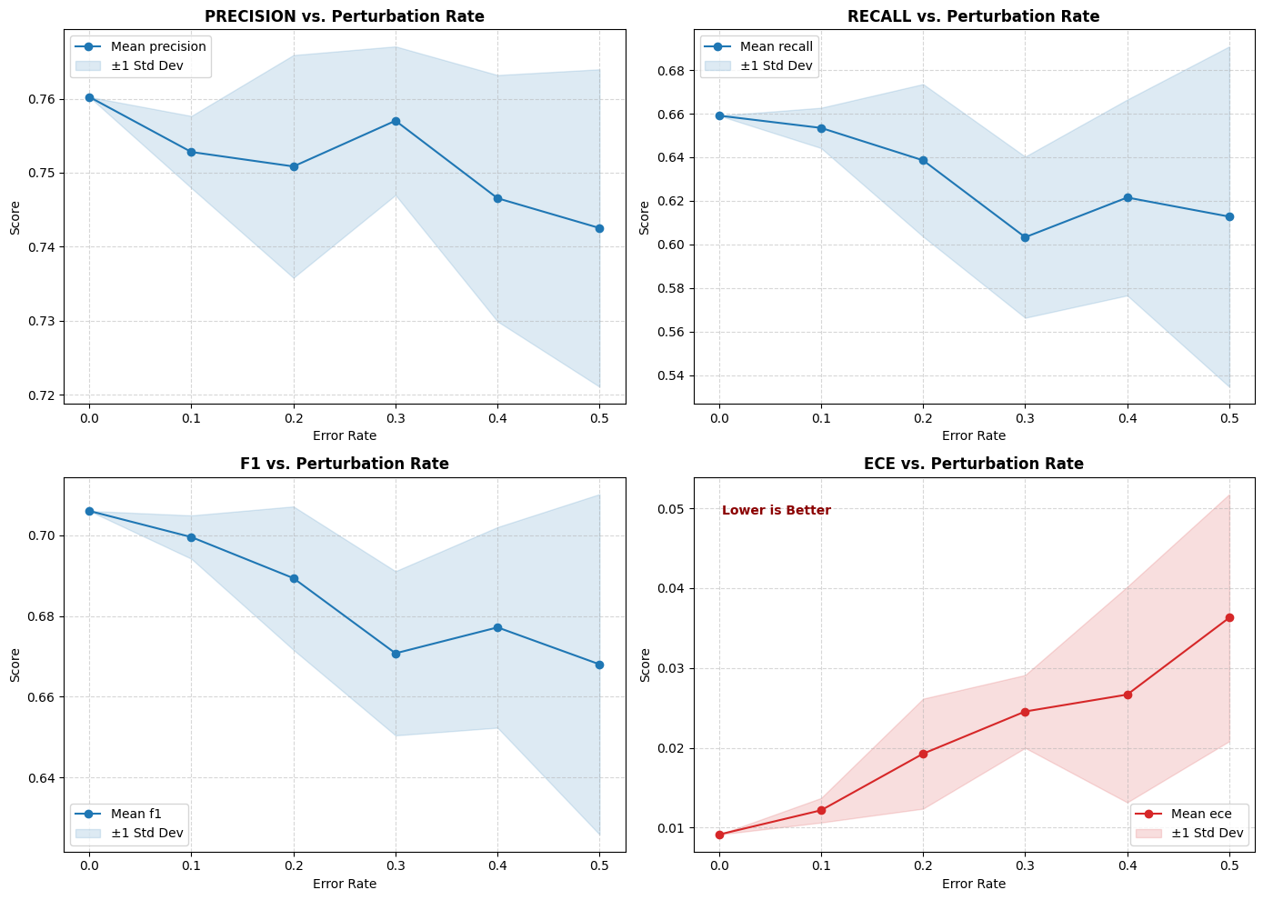

Fairness Evaluation¶

Motivation¶

Income prediction is used in credit scoring, hiring, and social programs. Biased models can systematically disadvantage protected groups.

Two leading fairness criteria:

Demographic Parity (DP): Equal positive prediction rates across groups $A \in \{a, b\}$ :

\Delta_{\text{DP}} = |P(\hat{Y}=1 \mid A=a) - P(\hat{Y}=1 \mid A=b)|

(9)

Equalized Odds (EO): Equal TPR and FPR across groups:

\Delta_{\text{EO}} = \max\bigl(|\text{TPR}_a - \text{TPR}_b|,\; |\text{FPR}_a - \text{FPR}_b|\bigr)

(10)

Reference: Hardt et al. (2016). Equality of Opportunity in Supervised Learning. NeurIPS.

Fairness Metrics — Further Definitions¶

Predictive Parity (Calibration within groups):

P(Y=1 \mid \hat{Y}=1, A=a) = P(Y=1 \mid \hat{Y}=1, A=b)

(11)

Impossibility theorem Chouldechova (2017): In the presence of base rate differences, DP, EO, and Predictive Parity cannot all hold simultaneously — practitioners must choose which to prioritise.

Sensitive attributes in Adult dataset:

sex: Male vs. Female
race: White vs. non-White (combined for power)

We use Fairlearn MetricFrame for disaggregated evaluation.

Chouldechova (2017)

# ── Fairlearn MetricFrame ─────────────────────────────────────────────────────
from fairlearn.metrics import (
    MetricFrame,
    demographic_parity_difference,
    equalized_odds_difference,
    selection_rate
)
from sklearn.metrics import accuracy_score, precision_score, recall_score

y_pred_main = pred_main.predict(X_test_main)

# Build sensitive features dataframe
sens = pd.DataFrame({
    'sex':  X_test_main['sex'].str.strip().values,
    'race': (X_test_main['race'].str.strip() == 'White').map(
                {True: 'White', False: 'Non-White'}).values
})

mf = MetricFrame(
    metrics={
        'accuracy':  accuracy_score,
        'precision': lambda y, yp: precision_score(y, yp, zero_division=0),
        'recall':    recall_score,
        'selection_rate': selection_rate
    },
    y_true=y_test_main.values,
    y_pred=y_pred_main.values,
    sensitive_features=sens
)

print(mf.by_group)

                  accuracy  precision    recall  selection_rate
sex    race                                                    
Female Non-White  0.948758   0.750000  0.489796        0.049689
       White      0.933843   0.808889  0.583333        0.086042
Male   Non-White  0.879459   0.827068  0.594595        0.163592
       White      0.843426   0.802013  0.666853        0.261541

# ── Aggregate disparity metrics ────────────────────────────────────────────────
dp_sex  = demographic_parity_difference(
    y_test_main.values, y_pred_main.values,
    sensitive_features=X_test_main['sex'].str.strip()
)
eo_sex  = equalized_odds_difference(
    y_test_main.values, y_pred_main.values,
    sensitive_features=X_test_main['sex'].str.strip()
)
dp_race = demographic_parity_difference(
    y_test_main.values, y_pred_main.values,
    sensitive_features=sens['race']
)
eo_race = equalized_odds_difference(
    y_test_main.values, y_pred_main.values,
    sensitive_features=sens['race']
)
print(f'DP(sex)={dp_sex:.4f}  EO(sex)={eo_sex:.4f}')
print(f'DP(race)={dp_race:.4f}  EO(race)={eo_race:.4f}')

def _plot_fairness():
    by_group = mf.by_group.reset_index()
    
    fig, axes = plt.subplots(1, 2, figsize=(12, 4))
    
    for ax, sens_feat in zip(axes, ['sex', 'race']):
        # Aggregate the MultiIndex to focus only on the current feature
        # This averages the metrics across the other sensitive categories
        grp = mf.by_group.groupby(level=sens_feat).mean()
    
        grp[['accuracy', 'selection_rate']].plot(
            kind='bar', 
            ax=ax,
            color=['#4C72B0', '#DD8452'],
            alpha=0.85, 
            rot=30
        )
        ax.set_title(f'Metrics by {sens_feat.capitalize()}')
        ax.set_ylim(0, 1)
        ax.set_ylabel('Score')
    
    plt.suptitle('Disaggregated Fairness Evaluation', fontsize=12)
    plt.tight_layout()
    plt.show()

DP(sex)=0.1705  EO(sex)=0.0895
DP(race)=0.0931  EO(race)=0.0818

_plot_fairness()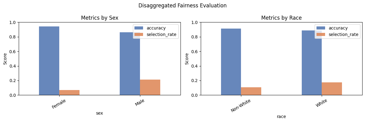

disparity = pd.DataFrame({
    'Demographic Parity Diff': [dp_sex, dp_race],
    'Equalized Odds Diff':     [eo_sex, eo_race]
}, index=['sex', 'race'])

fig, ax = plt.subplots(figsize=(7, 3.5))
disparity.plot(kind='bar', ax=ax, color=['#E53935','#1E88E5'],
               alpha=0.85, rot=0)
ax.axhline(0.1, ls='--', color='grey', label='Common 0.1 threshold')
ax.set_ylabel('Disparity (lower is fairer)')
ax.set_title('Fairness Disparity Metrics by Sensitive Attribute')
ax.legend(); plt.tight_layout(); plt.show()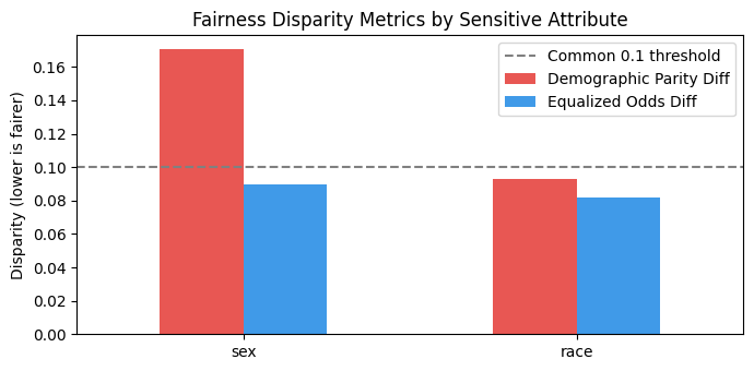

Fairness — Interpretation & Next Steps¶

Findings (typical on Adult dataset):

Sex: Female applicants are predicted >50K at a significantly lower rate than males even after controlling for other features — $\Delta_{\text{DP}} > 0.1$
Race: Non-White groups have lower TPR — $\Delta_{\text{EO}} > 0.05$

Mitigation strategies (not implemented here):

Pre-processing: Reweighing samples (Kamiran & Calders 2012)
In-processing: Fairness constraints in optimisation (Agarwal et al. 2018 — Fairlearn ExponentiatedGradient)
Post-processing: Threshold adjustment per group (Hardt et al. 2016)

Reference: Barocas, Hardt & Narayanan (2023). Fairness and Machine Learning. fairmlbook.org

Summary & Key Takeaways¶

Aspect	Key Tool	Key Finding
CV Evaluation	AutoGluon + StratifiedKFold	Reliable metric estimates with error bars
PR & Threshold	sklearn + custom loop	Target precision achievable at cost of recall
Feature Importance	AutoGluon permutation	`capital_gain`, `age`, `education_num` dominate
Calibration	sklearn + Isotonic Reg	Isotonic regression reduces ECE significantly
Energy	CodeCarbon	LightGBM best energy-accuracy ratio
Robustness	tab-err	Quantification of model robustness can be done with perturbations
Fairness	Fairlearn	Sex/race disparities exist; mitigation needed

Bottom line: Accuracy alone is insufficient. Responsible ML requires holistic evaluation.

References¶

Kohavi (1995). Study of cross-validation and bootstrap. IJCAI
Breiman (2001). Random Forests. Machine Learning, 45(1)
Davis & Goadrich (2006). PR vs ROC curves. ICML
Niculescu-Mizil & Caruana (2005). Good probabilities. ICML
Guo et al. (2017). Calibration of Neural Networks. ICML
Zadrozny & Elkan (2002). Multiclass probability estimates. KDD
Hardt et al. (2016). Equality of Opportunity. NeurIPS
Chouldechova (2017). Fair prediction with disparate impact. Big Data
Erickson et al. (2020). AutoGluon-Tabular. ICML AutoML Workshop
Courty et al. (2022). CodeCarbon. JMLR
Ovadia et al. (2019). Uncertainty under dataset shift. NeurIPS
Barocas, Hardt & Narayanan (2023). Fairness and ML. fairmlbook.org
Hooker & Mentch (2019). Stop Permuting Features. arXiv:1905.03151

References¶

Mitchell, M., Wu, S., Zaldivar, A., Barnes, P., Vasserman, L., Hutchinson, B., Spitzer, E., Raji, I. D., & Gebru, T. (2019). Model Cards for Model Reporting. Proceedings of the Conference on Fairness, Accountability, and Transparency, 220–229. 10.1145/3287560.3287596
Bouthillier, X., Delaunay, P., Bronzi, M., Trofimov, A., Nichyporuk, B., Szeto, J., Mohammadi Sepahvand, N., Raff, E., Madan, K., Voleti, V., Ebrahimi Kahou, S., Michalski, V., Arbel, T., Pal, C., Varoquaux, G., & Vincent, P. (2021). Accounting for Variance in Machine Learning Benchmarks. Proceedings of Machine Learning and Systems, 3, 747–769. https://proceedings.mlsys.org/paper_files/paper/2021/hash/0184b0cd3cfb185989f858a1d9f5c1eb-Abstract.html
Steinbach, P., Gernhardt, F., Tanveer, M., Schmerler, S., & Starke, S. (2022). Machine Learning State-of-the-Art with Uncertainties. arXiv. http://arxiv.org/abs/2204.05173
Kohavi, R., & others. (1995). A study of cross-validation and bootstrap for accuracy estimation and model selection. Ijcai, 14(2), 1137–1145.
Erickson, N., Mueller, J., Shirkov, A., Zhang, H., Larroy, P., Li, M., & Smola, A. (2020). AutoGluon-Tabular: Robust and Accurate AutoML for Structured Data. arXiv. 10.48550/arXiv.2003.06505
Davis, J., & Goadrich, M. (2006). The relationship between Precision-Recall and ROC curves. Proceedings of the 23rd International Conference on Machine Learning, 233–240.
Lipton, Z. C., Elkan, C., & Naryanaswamy, B. (2014). Optimal thresholding of classifiers to maximize F1 measure. Joint European Conference on Machine Learning and Knowledge Discovery in Databases, 225–239.
Guo, C., Pleiss, G., Sun, Y., & Weinberger, K. Q. (2017). On Calibration of Modern Neural Networks. arXiv. 10.48550/arXiv.1706.04599
Lottick, K., Susai, S., Friedler, S. A., & Wilson, J. P. (2019). Energy Usage Reports: Environmental awareness as part of algorithmic accountability. arXiv Preprint arXiv:1911.08354.
Jung, P., Jäger, S., Chandler, N., & Biessmann, F. (2025). Towards realistic error models for tabular data. ACM Journal of Data and Information Quality, 17(4), 1–27.
Chouldechova, A. (2017). Fair prediction with disparate impact: A study of bias in recidivism prediction instruments. Big Data, 5(2), 153–163.